PART 4 : Position Estimation.
- Table of contents
- PART 4 : Position Estimation.
Once the navigation bits from at least 4 satellites have been retrieved from the acquisition/tracking part, it is possible to estimate the desired position of the receiver.
1 - Ephemeris.
GPS uses a particular algorithm in order to characterise satellite position. In comparison with GLONASS, this method requires more parameters, but less complexity.
a - Introduction of satellite orbit from [2].
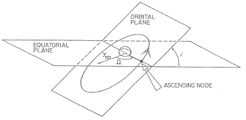
Figure 4.1 : Orbital plane positioning.
Orbital plane positioning parameters :
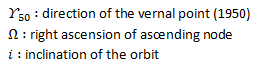
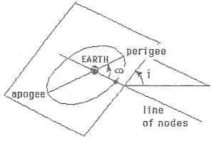
Figure 4.2 : Orbit positioning in the orbital plane.
Orbit positioning in the orbital plane :

Figure 4.3 : Orbital plane positioning.
Shape of the orbit :
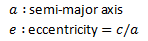
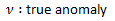
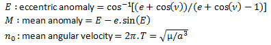
Positioning of the satellite on the orbit :
Induced parameters :
b - GPS satellite ephemeris data.
GPS uses previous classical ephemeris data for orbit and satellite position determination, and decompose them into elementary parameters to be implemented in the navigation frame :
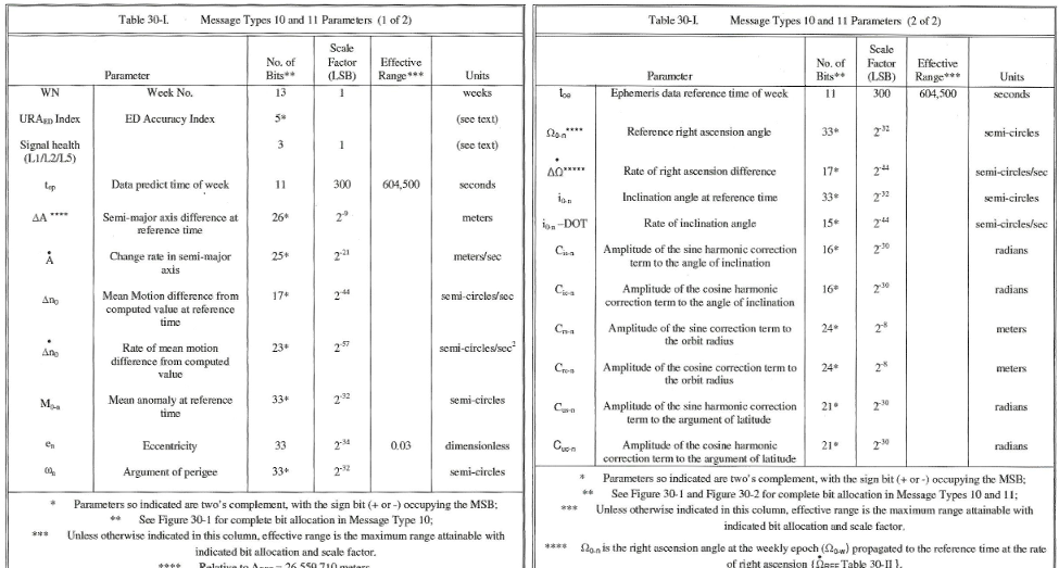
Figure 4.4 : List of ephemeris parameters included in GPS frames.
c - GPS satellite position calculation algorithm.
Starting from the GPS ephemeris present in the navigation frame - subframes 2 and 3 - it is now possible to compute the satellite position via the following algorithm :
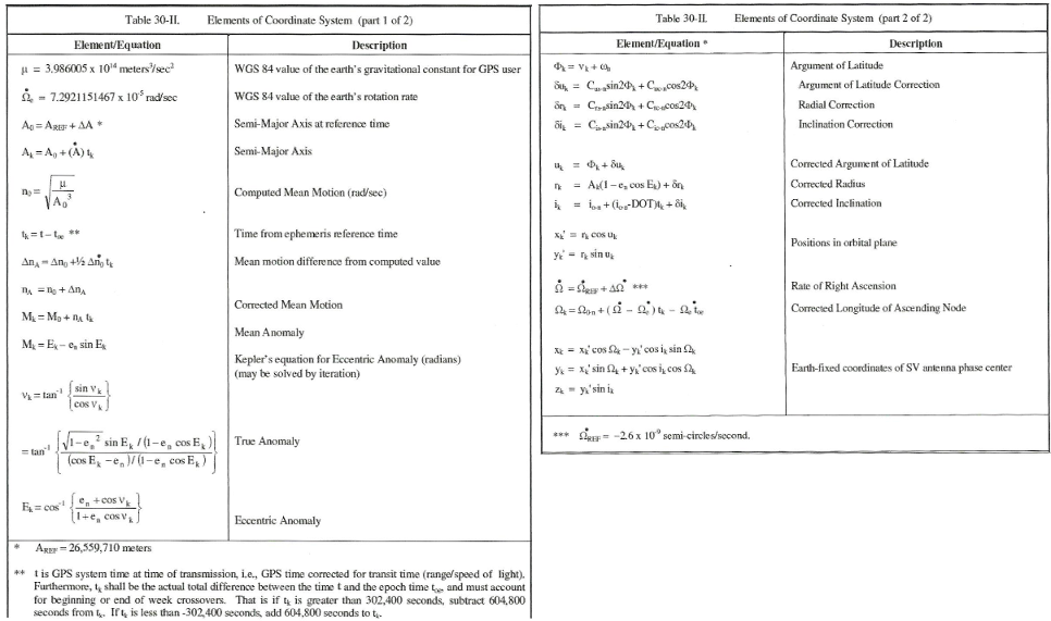
Figure 4.5 : Description of the algorithm step by step.
These tables are extracted from GPS Interface Control Document [3]
2 - Navigation computation.
a - Reminder about the range impairments.
The following figure gives the impairments affecting the range in case of the GPS system as well as the correction process :
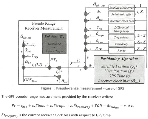
Figure 4.6 : Pseudo-range measurement extracted from [4]
b - Demonstration of the Pseudo-ranges with Least Square method.
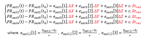
Starting from the fact that can determine most of the elements within the pseudo-range measurement PR_sat(i) from the information provided by each satellite, we have the equation :

Equation 1
or put in another way,
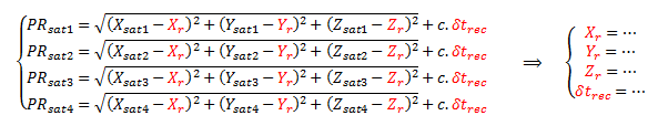
Equation 2
Indeed 4 measurements are needed, providing 4 equations with 4 unknows which are the receiver coordinates and the clock bias of the receiver. As the equation is highly non-linear, it is important to proceed to a linearization such as the Taylor expansion :
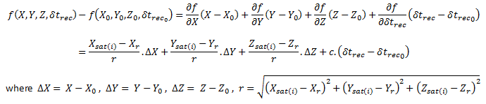
Equation 3
Hence,
Equation 4
In practise, for a receiver located e.g. in France PR (t_0) can be described by Paris location as initialization for the algorithm.
In vectorial form the equation becomes :
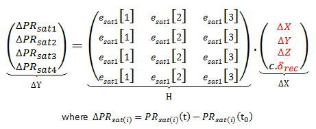
Equation 5
which can be expressed as :
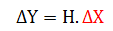
Equation 6
with the Least Square solution :
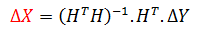
Equation 7
Thus, it is possible to retrieve the receiver position.
Note that all unknowns are depicted in red color.
c - Kalman filter.
Another position estimation method is Kalman filter i.e. an algorithm that uses a series of measurements observed over time, containing statistical noise and other inaccuracies, and produces estimates of unknown variables that tend to be more precise than those based on a single measurement alone.
In this project, a single measurement will be used for "simplicity" purposes, therefore, the Least Square method is more appropriate for this issue.
References :
[1] K. Borre, D. M. Akos, N. Bertelsen, P. Rinder, S. H. Jensen, A software-defined GPS and GALILEO receiver
[2] M. Bousquet, Orbits and Satellite Platforms lecture script, January 2016
[3] GPS Interface Control Document under http://www.gps.gov/technical/icwg/IS-GPS-200H.pdf
[4] Position Estimation Workshop, March 2016
