
LabVIEW implementation
Why LabVIEW?
The first step of the project consists in designing a communication system based on the QPSK modulation. The implementation of the QPSK communication system is developed in LabVIEW. LabVIEW is a software development environment that contains numerous components and tools for building a wide variety of applications. It also allows to integrate hardware devices to the designing such as sensors, cameras, data acquisition devices, etc.
This feature is very useful because later we will replace the transmitter and receiver of the communication system with real DVB-S2 modems. This allows us to verify firstly the correct operation of the developed system and then to replace progressively their components.
In particular we will use the LabVIEW Modulation Toolkit which provides several examples using QPSK modulation. We will use one of these examples as a starting point to develop our QPSK communication system. On the other hand, LabVIEW provides a FPGA Module which provides a graphical development platform for FPGA.
The LabVIEW example
The selected example implements an Offset QPSK transmitter/receiver system which is a variant of the normal QPSK modulation in order to make much lower amplitude fluctuations in the transmitted signal. As shown in Figure 3, the front panel is the user interface that contains the controls and indicators of the simulation. The block diagram implementation of the QPSK communication system is shown in Figure 4.
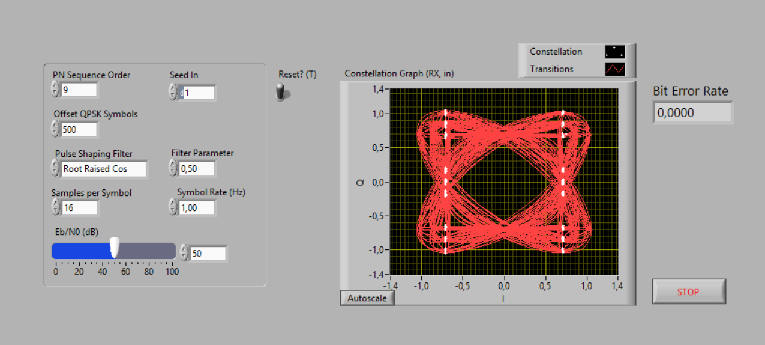
Figure 3 Front panel of the LabVIEW example
In the front panel, the user can modify the main simulation parameters such as the transmission filter, the roll-off factor, the signal to noise ratio (Eb/N0), etc. To analyze the simulation results the front panel also plots the eye diagram at the receiver output and displays the bit error rate. The user can vary the simulation parameters and see how it impacts on the transmission performance in real time.
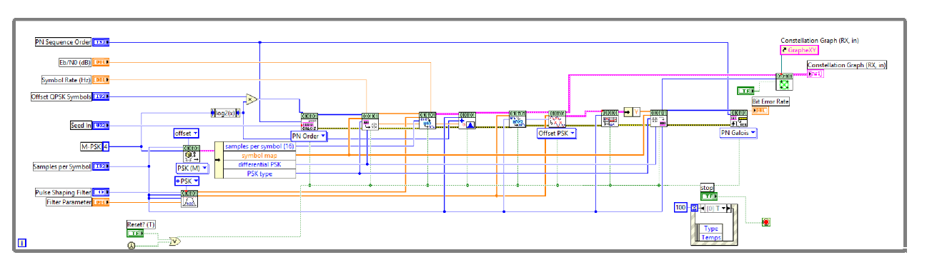
Figure 4 Block diagram of the LabVIEW example
As shown in the diagram block, the program consist of one big while loop in which a data signal is modulated for transmission and demodulated for reception. We describe succinctly the operation of this communication system. At each iteration, a bit sequence is generated and mapped to QPSK symbols. Then, the signal is filtered and transmitted to the channel where white gaussian noise is added to the signal. Finally, the received signal is matched filtered and sampled to estimate the transmitted symbols.
Since all the performed operations are in the same while loop, it becomes problematic to replace and integrate other transmitters and receivers. Therefore, in order to develop a suitable QPSK communication system for our purposes the following steps must be performed:
- Understand the performed operations (creating a bit secuence, mapping to symbols, filtering, etc) in the example to simulate the QPSK modulation.
- Identify the operations corresponding to the transmitter, the channel and the receiver.
- Modularize the communication system scheme in order to separate the transmitter, the channel and the receiver.
- Find a way to connect the created modules to replace them easily.
- Implement the delay effect on the new scheme.
Our LabVIEW implementation
In this section, we develop our QPSK communication system using LabVIEW tools. For the implementation, we use the complex envelope representation of the signal in the transmission and reception. Since the complex envelope signal can be represented using a much smaller sampling rate than the corresponding passband signal, the computational cost is lower.
We now describe the components of the communication system and its operation. Figure 5 shows the block diagram of the developed system. As shown in the diagram, the whole communication system has been divided into three loops, each one of them is corresponding to the transmitter, the channel and the receiver. In order to connect these loops, we use a queue to buffer the output generated by one loop. Then, at each iteration the next loop takes one element of the queue as an input to process it.
The QPSK signal is generated in the transmitter loop. At each iteration, the transmitter loop generates a cluster containing an array with samples of the complex envelope transmitted signal, the time interval is between samples in the array and the start time of the array. This cluster is stored in a queue.
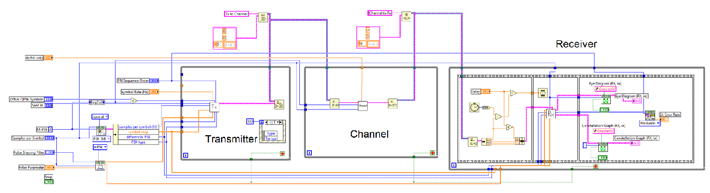
Figure 5 Block diagram of the developed system
The channel loop removes the cluster from the queue to process it. In this loop, complex white gaussian noise is added to the signal at a given SNR level which is selected by the user. As in the previous case, a cluster contains an array with samples of the noisy signal, the time step and the star time is stored in a queue.
Finally, the receiver loop subtracts the cluster from the second queue and performs two main operations:- a time delay is introduced in the signal by modifying the start time of the cluster.
- the received signal is filtered and decimated to estimate the transmitted symbols.
The main simulation parameters are: a) The SNR level; b) The time delay; c) The number of samples per symbol; d) The symbol rate; e) The shape of the transmitter filter; f) The roll-off factor for the raised cosine filter. The users can modify these parameters by using the front panel as shown in Figure 6. The front panel also displays the received symbol constellation, the eye diagram at the output receiver and the bit error rate.
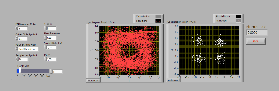
Figure 6 The modified front panel includes a control to select the delay and shows the received constellation
This approach using three loops and two queues to connect them allows us to replace easily one of the system components by another component. For instance, in this project we will replace the transmitter and receiver loops with real DVB-S2 modems.
We now explain the details of each of the communication system loops. As shown in Figure 7, the first one is the transmitter loop which is composed of three blocks:- MT Generate Bits: This block generates the sequence of data bits to be modulated. It generates Galois pseudonoise bit sequences.
- MT Map Bits to Symbols: This block maps bits to complex valued symbols for QPSK modulation.
- MT Pulse Shaping Filter: This block generates a sampled continuous time QPSK baseband signal from the discrete-valued input symbols by applying a pulse shaping filter.
Finally, we include the start time of the generated signal by getting the current time and adding it to the cluster.
![]()
Figure 7 Transmitter block
Figures 8 shows the scheme of the channel block which generates zero-mean complex additive white gaussian noise and adds it to the complex baseband modulated waveform.
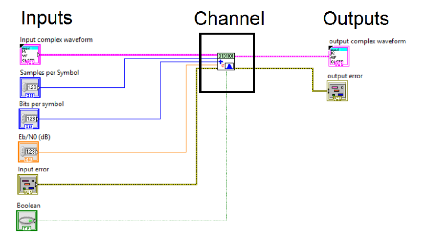
Figure 8 Channel block
It is important to notice that the delay effect is not implemented in the channel loop but in the receiver loop. The delay is selected by the user by using the front panel and it takes into account that the processing time is between the transmitter output and the receiver input. For instance, the delay effect comprises the waiting time in the queues and channel processing time.
Figure 9 shows the diagram of the receiver block. Here we explain the operations performed in the sub-blocks:- MT Matched Filter: This block applies the corresponding matched filter to the received complex QPSK baseband signal. The fact of filtering the received signal with the matched filter of the transmitter filter maximizes the signal to noise ratio. In addition, since the transmitter filter is the root raised cosine filter, the communication system satisfies the Nyquist condition.
- MT Align To Ideal Symbols: This block aligns the first sample of the received complex signal to the ideal symbol timing instant which the signal to noise is maximum.
- MT Decimate Oversampled Waveform: This block decimates the matched filtered signal. The downsamplig allows to recover the transmitted symbols of the signal.
- MT Map Symbols to Bits: This block estimates the QPSK received symbols and generates an output bit stream.
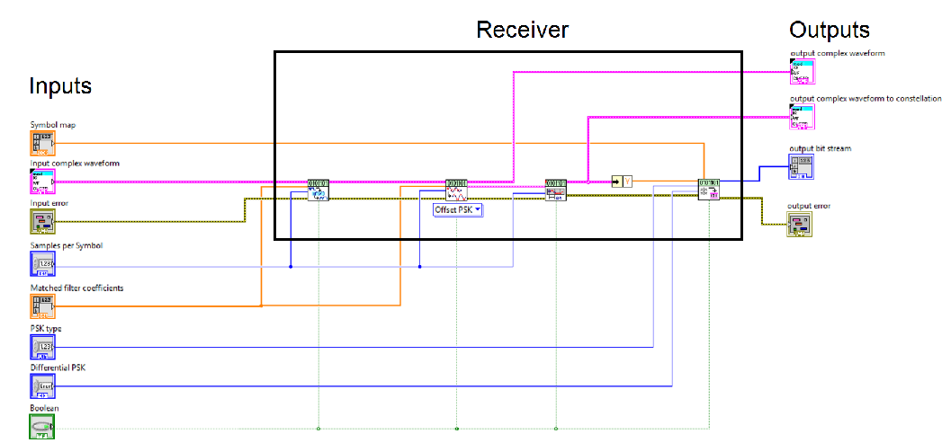
Figure 9 Receiver block
Test and results
Finally, we analyze the performance by comparing with theoretical results. We plot the BER vs Eb/N0 curve in order to validate our implementation. As shown in Figure 10, the red curve represents the theoretical values while the blue corresponds to the results in practice. It is mentioned that the obtaining results match with the theoretical ones. Therefore, the developed implementation is suitable for our project requirements
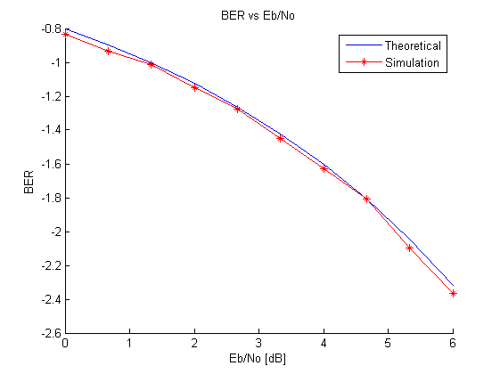
Figure 10 BER vs Eb/N0