
Performance analysis and results
Several tests are carried out in order to evaluate the performance of the developed channel emulator. Firstly, it must be verified that the required $Eb/No$ level is achieved at the demodulator output. Secondly, the time delay of transmitted packets must be measured to guarantee compliance with the specified delay.
Noise measurements
Consider the test bench shown in Figure 1 in order to measure $Eb/No$ level during the transmission. The hub modem sends a QPSK modulated signal to the station modem through the satellite channel represented by the VST. Then, the channel-applied signal is received at the demodulator input of the station modem where the $Eb/No$ measurement is performed. The carrier-to-noise power can be obtained in two different ways by using the monitoring tools of the modem or the spectrum analyzer.
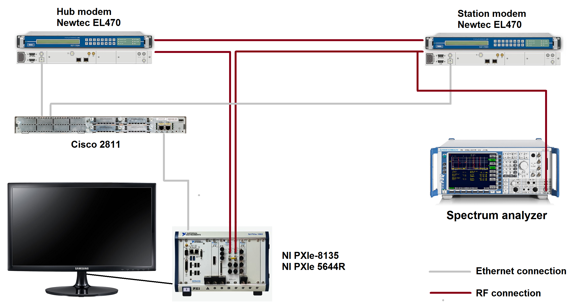
Figure 1. Test bench used to measure $Eb/No$
A first approach consist of using the monitoring tools included in the modem configuration interface. Figure 2 shows the measured carrier-to-noise power over 2 minutes for 0 dB, 5 dB, 10 dB, 15 dB, 20 dB and 50 dB. As can be observed the obtained values are approximately the same as the selected $Eb/No$ values in the front panel of the emulator. It can be noticed that for 0 dB, the demodulator is not capable to demodulate the QPSK signal and recover the received IP packets as shown in Figure 3 where the IP throughput for 5 dB and 0 dB are plotted.
Furthermore, as can be seen in Figures 2(e) and 2(f), the obtained carrier-to-noise value is around 16.5 dB while the required $Eb/No$ values are 20 dB and 50 dB. Therefore, it means that there is an upper bound in the $Eb/No$ that can be generated by the channel emulator. Since the modems are connected through an active device, the noise power level is increased according to the VST noise figure and, therefore, the carrier-to-noise power is degraded.
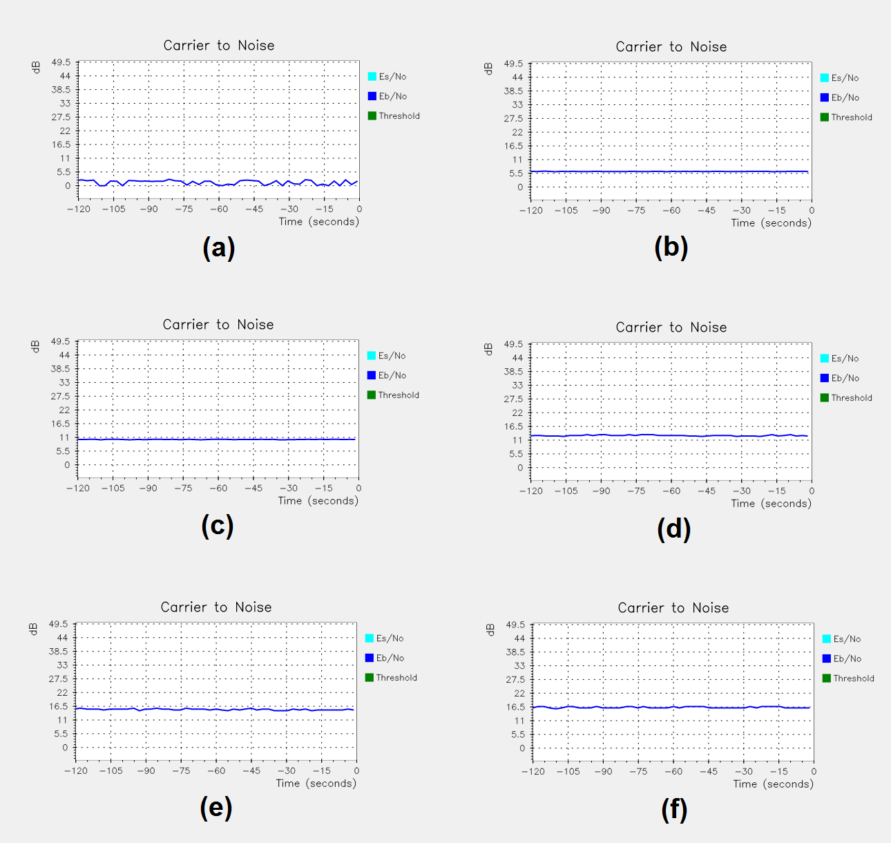
Figure 2. $Eb/No$ measurements obtained from the modem interface. Selected $Eb/No$ value: (a) 0 dB;(b) 5 dB;(c) 10 dB;(d) 15 dB;(e) 20 dB and (f) 50 dB
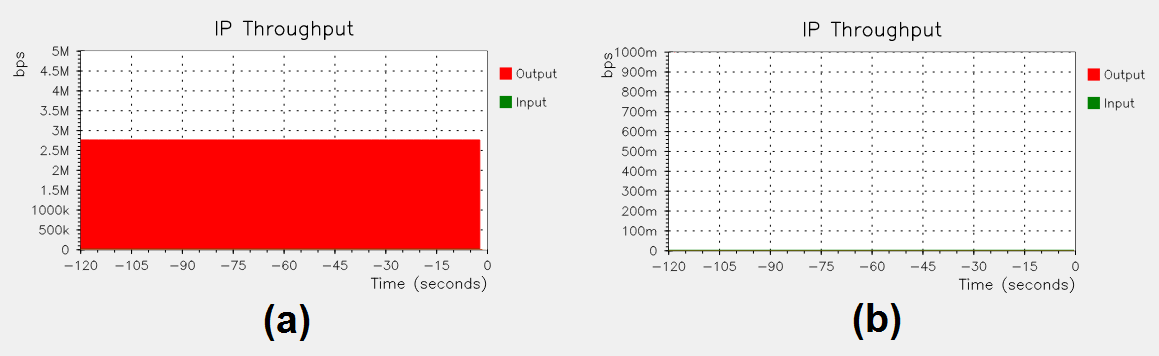
Figure 3. IP throughput for 5 dB and 0 dB
In order to analyze the impact of the channel emulator on the noise power level, the following measurements are performed: the carrier-to-noise power ratio when the modems are directly connected between them and the carrier-to-noise power when the VST is included in the transmission chain but without performing any signal processing, i.e., adding noise or including time delay.
As can be seen in Figure 4(a), the carrier-to-noise ratio is around 22 dB when the VST is not connected, which means that the channel emulator is constrained to produce a maximum $Eb/No$ value below 22 dB. On the other hand, even if the channel emulator is not adding noise to the QPSK signal, the carrier-to-noise is reduced by 5.5 dB as can be observed in Figure 4(b). Therefore, the channel emulator is limited to deliver a signal whose $Eb/No$ value is below 16.5 dB.
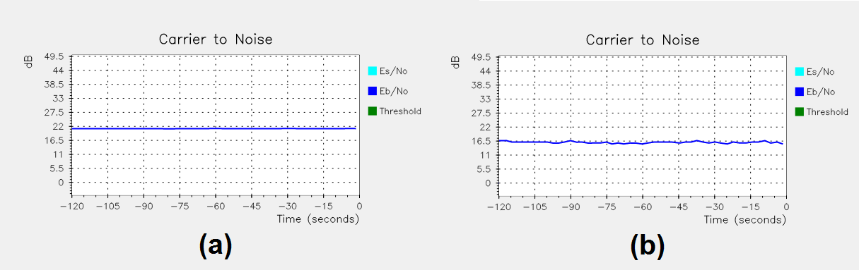
Figure 4. $Eb/No$ degradation introduced by the emulator
In addition, it can be seen how the transmitted signal is affected by the emulator channel by using the modem interface which also provides information about the power in dBm of the received signal. The received power level when the channels are directly connected is equal to -44 dBm (Figure 5(a)) while it is equal to -62 dBm (Figure 5(b)) when the VST is included in the transmission chain without performing any signal processing. In Figure 5(c), it can be observed the load effect of the spectrum analyzer on the received power, the fact of disconnecting the spectrum analyzer from the test bench generates an increase of 6 dB in the received power.
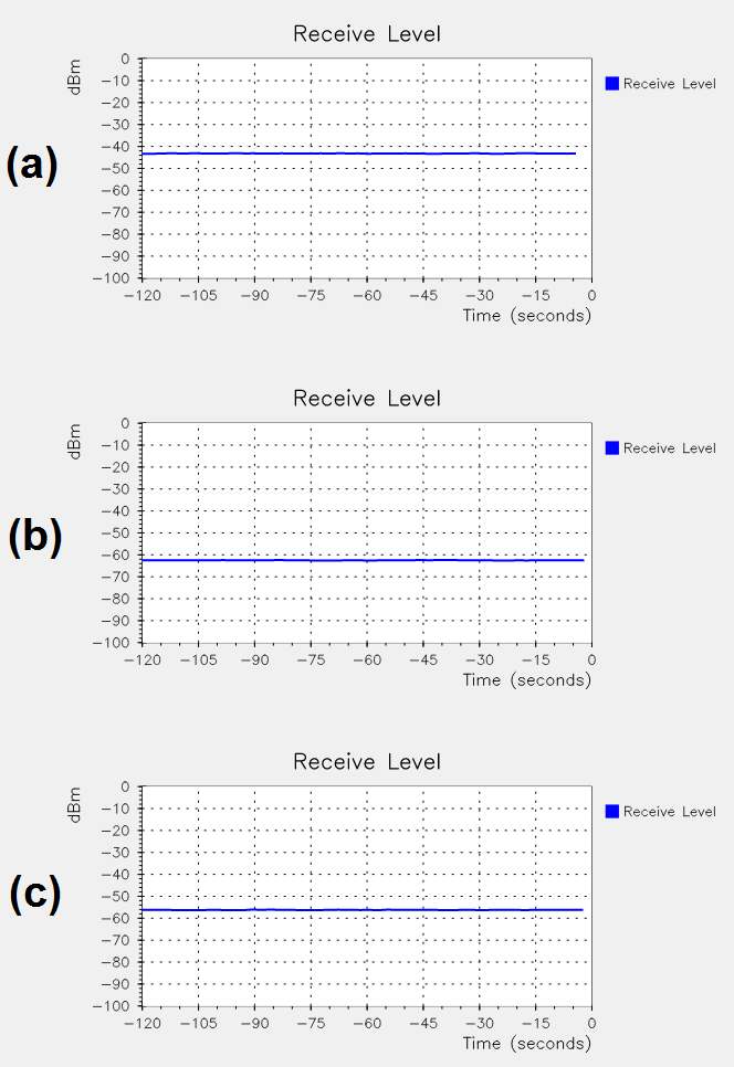
Figure 5. Output power degradation introduced by the emulator
Another approach to evaluate the channel emulator performance is studied here. A spectrum analyzer is connected via a coaxial cable to the input of the station modem. The spectrum analyzer plots the frequency response magnitude of the channel-applied signal as illustrated in Figure 6. Given that the signal power as well as the noise power can be measured with the spectrum analyzer, the signal-to-noise ratio can be computed and, subsequently, the $Eb/No$ can be deduced from the following formula
$SNR = Eb/No . Rb/B$$
By using the spectrum analyzer, the frequency response magnitude at the demodulator input is obtained for 0 dB, 5 dB, 10 dB, 15 dB, 20 dB and 50 dB. Given that only the noise power is modified, as the $Eb/No$ value is increased by 5 dB (see Figures 6(a), (b), (c), (d) and (e)), the noise power is reduced by the same amount without modifying the signal power which validates the noise generation implementation.
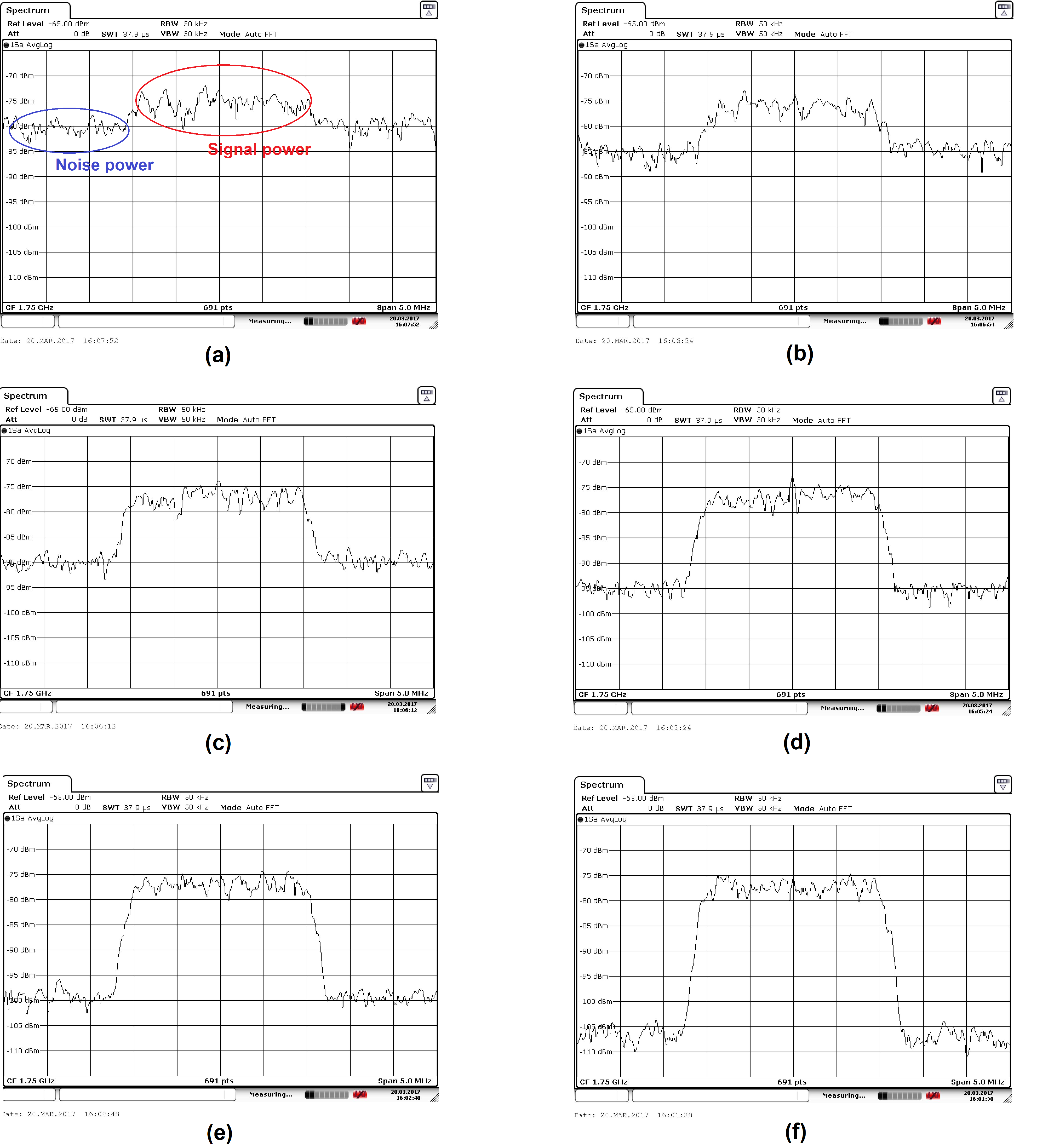
Figure 6. Signal-to-noise power measurements carried out with the spectrum analyzer. Selected $Eb/No$ value: (a) 0 dB;(b) 5 dB;(c) 10 dB;(d) 15 dB;(e) 20 dB and (f) 50 dB
As in the previous case, the impact of the VST in the channel emulation is examined by the spectrum analyzer. In Figure 7, a 20 dB difference in the received signal power as well as an increase in the noise power can be observed when the channel emulator is connected to the modems.
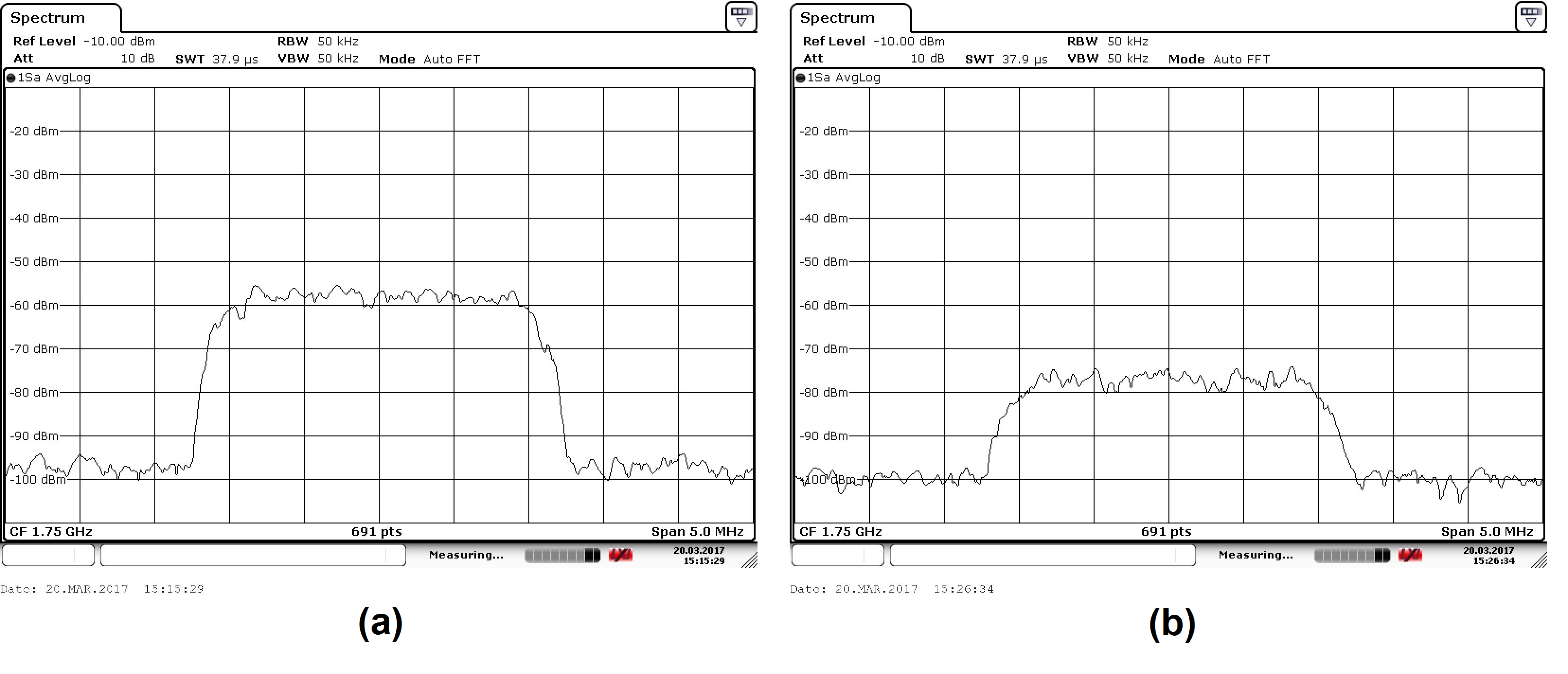
Figure 7. Signal power degradation due to the emulator
Delay measurements
For the purpose of measuring the time delay through the channel, the ping command is used in our approach. The ping command is typically used to verify that a computer can communicate over the network with another computer or network device. ICMP Echo Request messages are sent to the target computer which answers by sending ICMP Echo Reply messages that provide information about the round trip time delay.
Firstly, the VST is not included in the architecture, i.e., the modems are connected back-to-back as can be seen in Figure 8, in order to measure a reference round trip time. A ping command is executed sending 10 ICMP Echo Request containing 1 bytes and 1500 bytes of data, the results are respectively displayed in Figure 9. Two packet sizes are used to analyze the propagation time in the satellite channel.
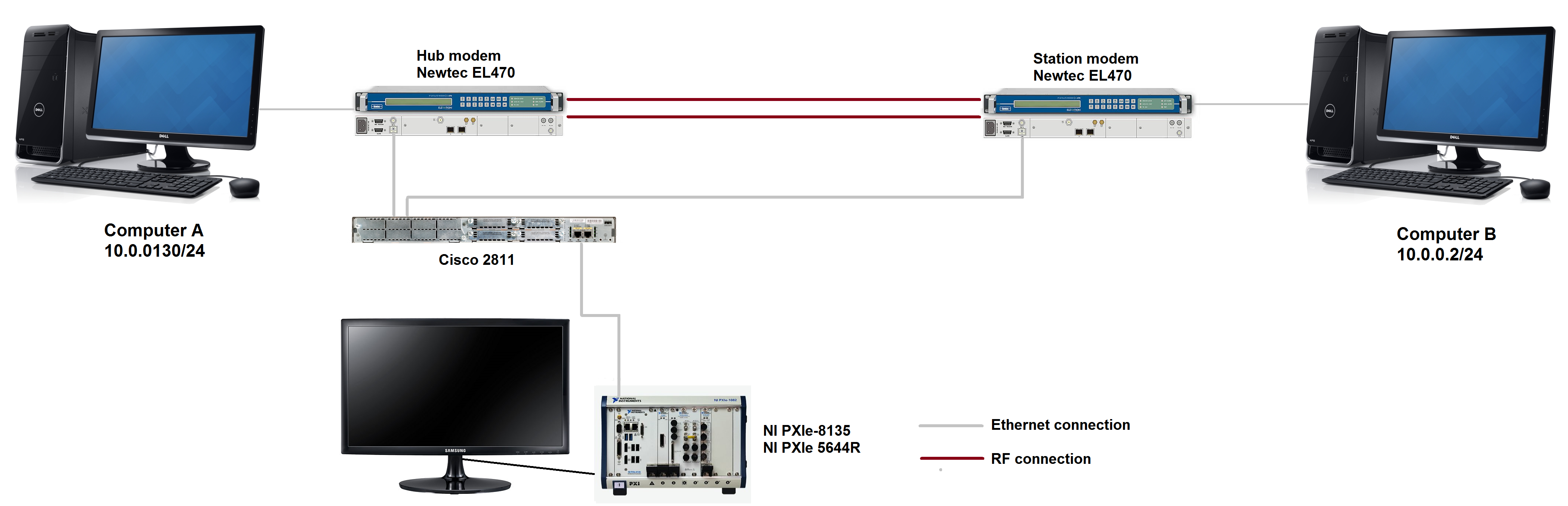
Figure 8. Test bench used to measure a reference round trip time
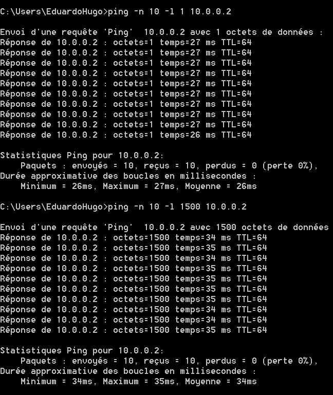
Figure 9. Round trip time measurements using the ping command (10 packets of 1B and 1500B, respectively) when the emulator is not connected
The average round trip time delay for the transmission of 1 bytes and 1500 bytes are respectively 26 ms and 34 ms. As expected, as the packet size is increased the round trip time delay is also increased due to the network processing.
Figure 10 depicts the test bench to determine the round trip time delay when the channel emulator is included in the architecture. As in the previous case, a ping command is executed sending 10 ICMP Echo Request which contain 1 bytes and 1500 bytes of data. Assuming that the propagation time in the SMA and coaxial cables are negligible ($t_{prop} \inf 1\mu s$), the time difference with respect to the reference round trip time provides the delay introduced by the channel.
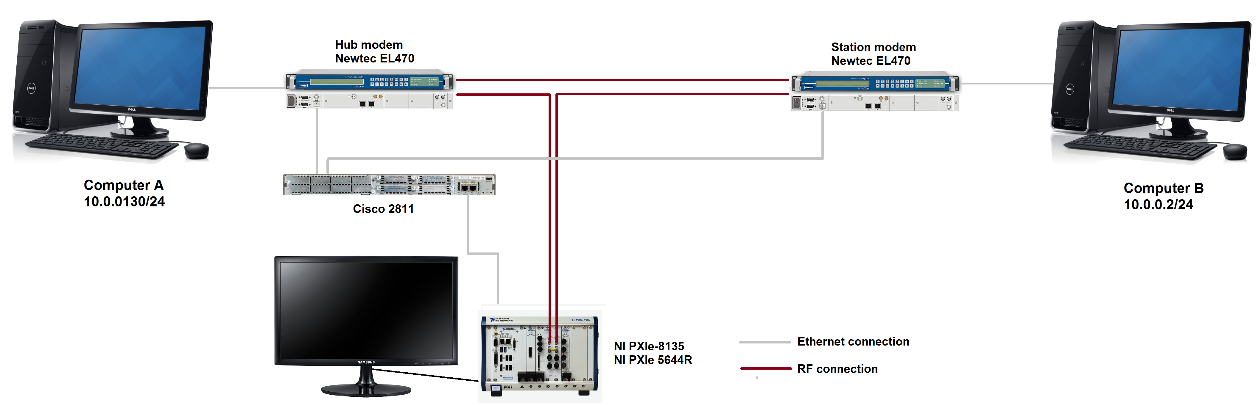
Figure 10. Test bench used to measure the total round trip time
The first measurements are performed considering a delay of 0 ms in order to estimate the signal processing carried out in the VST. In addition, to verify the time delay implementation, the ping command is executed for 50 ms, 100 ms, 150 ms and 200 ms delay values, the results are shown in Figures 11 and 12 and summarized in Table 1 and 2.
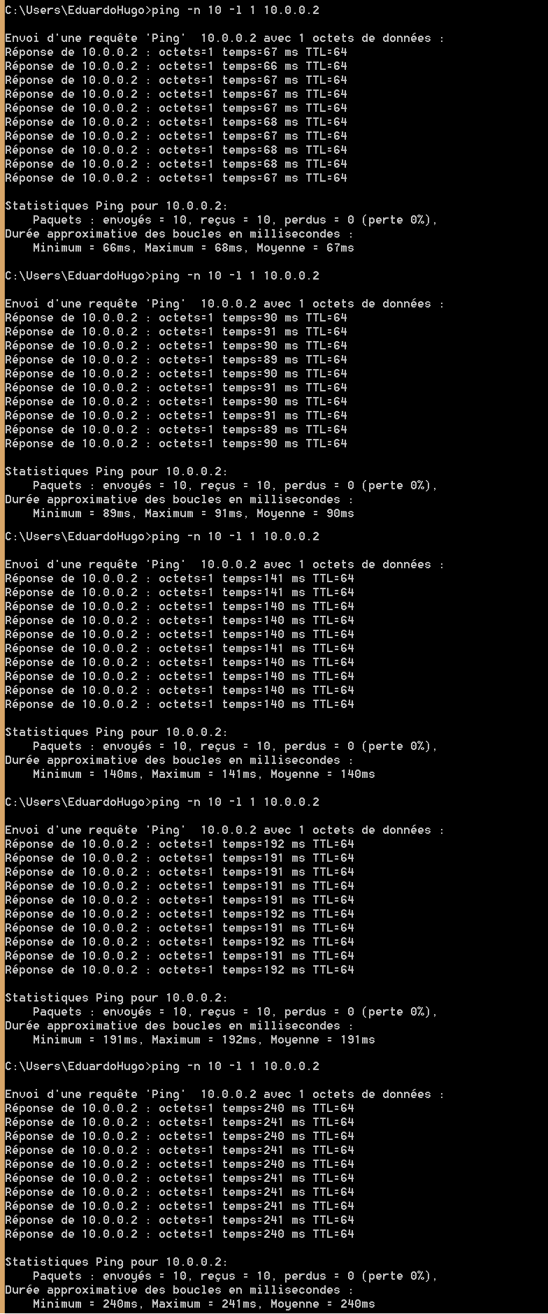
Figure 11. Round trip time measurements using the ping command (10 packets of 1B) when the emulator is connected for different delays values
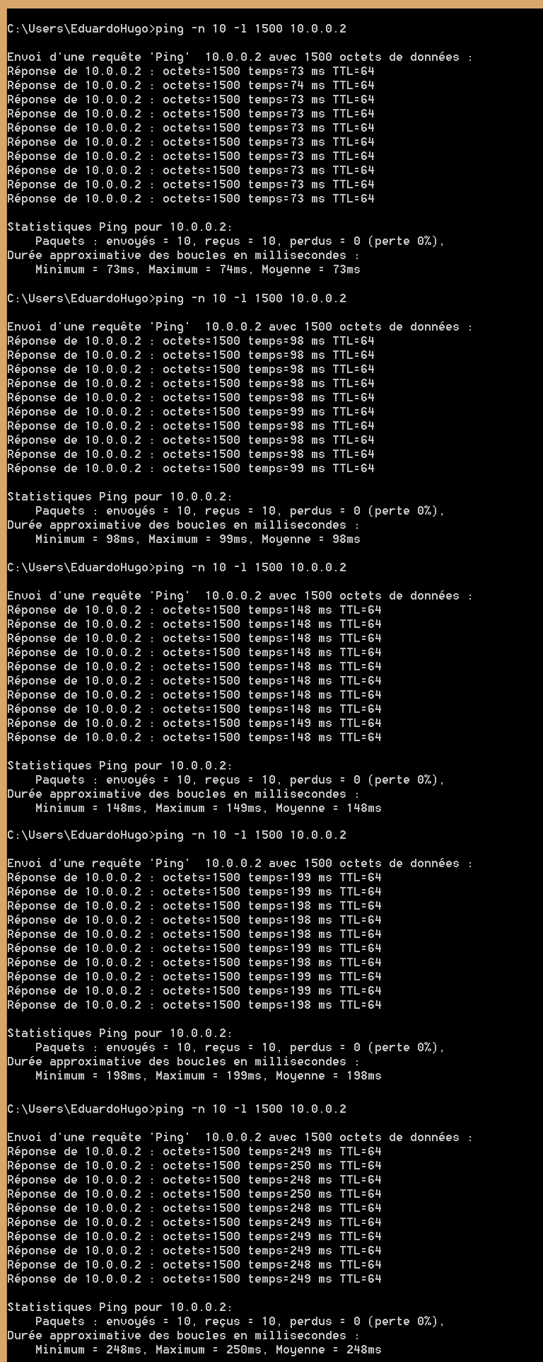
Figure 12. Round trip time measurements using the ping command (10 packets of 1500B) when the emulator is connected for different delays values
The tables summarizes the most significant values obtained from the measurements. The time $t_d$ corresponds to the selected time delay in the front panel, $t_{RTT}$ represents the measured round trip time, t_i represents the effective time delay introduced by the channel emulator and $t_{diff}$ represents the difference between the effective time delay and the selected time delay. For values higher than 50 ms, $t_{diff}$ remains constant and, therefore, the delay introduced by the channel behaves linearly with respect to the selected time delay as shown in Figure 13.
| Time delay $t_d$ | Average RTT $t_{RTT}$ | Delay introduced $t_i = t_{RTT} - t_{net}$ | Delay difference $t_{diff} = t_i - t_d$ |
|---|---|---|---|
| 0 ms | 67 ms | 41 ms | 41 ms |
| 50 ms | 90 ms | 64 ms | 14 ms |
| 100 ms | 140 ms | 114 | 14 ms |
| 150 ms | 191 ms | 165 ms | 15 ms |
| 200 ms | 240 ms | 214 ms | 14 ms |
Table 1. Delay measurement summary (1 bytes transmitted)
| Time delay $t_d$ | Average RTT $t_{RTT}$ | Delay introduced $t_i = t_{RTT} - t_{net}$ | Delay difference $t_{diff} = t_i - t_d$ |
|---|---|---|---|
| 0 ms | 73 ms | 39 ms | 39 ms |
| 50 ms | 98 ms | 64 ms | 14 ms |
| 100 ms | 148 ms | 114 ms | 14 ms |
| 150 ms | 198 ms | 164 ms | 14 ms |
| 200 ms | 248 ms | 214 ms | 14 ms |
Table 2. Delay measurement summary (1500 bytes transmitted)
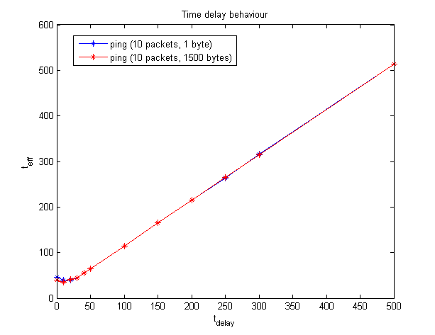
Figure 13. Time delay behaviour