
1. Definition of inputs and ways to compute the outputs - Theory
1. Display of the power spectrum

Figure 9: Computation of the Power Spectrum
The incoming signal passes through the "power spectrum block" of LabView. The power spectrum of the given signal is then displayed.
2. Computation of the power of the useful signal

Figure 10: Computation of the Power of the useful signal
The value of the autocorrelation of the signal taken at 0 gives the total power of the signal. If the signal is noisy, the result will be the power of the useful signal added to the one of the noise. Generally, the power of the useful signal is much higher than the power of the noise. Therefore, this model is valid when the power of the noise is much lower than the one of the useful signal. This model is only valid for the simulation, it will be modified in subsection 3. Moving from simulation to acquisition of real signals.
3. Computation of the power of the noise
The noise will be known for the simulation, therefore, its power will be known and the signal-to-noise ratio will be approximated by dividing the measured power of the useful signal by the power of the noise.
4. Display of the constellation

Figure 11: Display of the constellation
The signal is demodulated with the appropriate demodulation parameters (see subsection 4. Signals to be measured for the definition of the parameters).
5. Computation of the error measurements
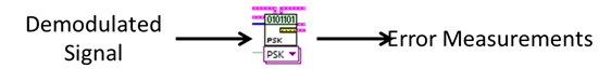
Figure 12: Error Measurements