
PART3 » History » Version 79
« Previous -
Version 79/83
(diff) -
Next » -
Current version
COLIN, Tony, 03/23/2016 12:08 PM
PART 5 : Implementation and results.
- Table of contents
- PART 5 : Implementation and results.
This part is dedicated to explain and illustrate the main steps that have been done in order to retrieve a navigation signal and to compute the position of the receiver from the pseudo-range measurements of 4 satellites. PART 2, PART 3 and PART 4 provided a theoretical background on GPS signals, the main blocks of a GPS receiver and methods to compute the position using the navigation data. Now, it is time to put this theoretical knowledge into practice.
As lots of VIs have been created, a UML diagram has been drawn to illustrate the structure of the overall code. For each main step that will be described, a link to the UML diagram will be provided, the different VIs to be taken into consideration will be listed, a few key points regarding the implementation will be clarified and the results will be displayed.
1 - Starting point.
a - Quid about LabVIEW.
Labview is a modular dataflow programming language that relies on block diagrams interconnected with each other. Each block diagram represents a node, a function that can be run as soon as its inputs are available. Then, it computes outputs used as inputs by other nodes. Any created program can be reused as a node in a higher-level program, hence the modularity of Labview. While running a program, each input can be controlled thanks to a user interface known as a “front panel”. Likewise, every output can be monitored and displayed using the front panel. As a matter of fact, the front panel is closely linked to the program called the “block diagram”. Indeed, every primary input of the block diagram are defined and controlled via the front panel.
b - Receiver scheme and milestones.
The software-defined GPS receiver to be implemented should take as an input a sampled signal that has been received and down-converted by an RF receiver front-end. As our RF receiver front-end was missing an antenna, we used a recorded GPS raw signal from the output of an RF front end (from CD [1] under GNSS_signal_records/GPSdata-DiscreteComponents-fs38_192-if9_55.bin). In order to read properly the data that are contained in the recorded file, one needs to know the sampling frequency and the intermediate frequency of the raw signal.
Sampling frequency = 38.192 MHz
Intermediate frequency = 9.55 MHz
The following diagram sums up the general structure of the GPS receiver to be implemented.
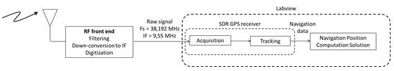
Figure 5.1: General receiver scheme.
c - Local C/A code generation.
The files involved are :
- CA_Code.vi : SnapCACode.png
- CA_generatorG1.vi : SnapG1.PNG
- CA_generatorG2.vi : SnapG2.png
These VIs allow generating a PRN sequence according to the satellite ID and the sampling frequency. Indeed, the newly generated PRN sequence has to be multiplied with the incoming signal. Knowing that the period of one PRN sequence is 1 ms, the length of the generated sequence has to be adjusted according to the sampling frequency. With a sampling frequency of 1.023 MHz, a sampled PRN sequence with 1023 samples is generated. With a sampling frequency of 38.192 MHz, a sampled PRN sequence with 38192 samples is generated.
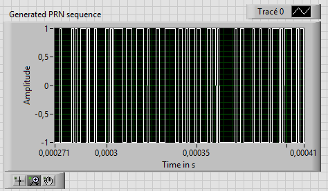
Figure 5.2: Example of a locally generated PRN sequence.
In Figure 5.2, a PRN sequence corresponding to satellite 21 has been generated with a sampling frequency of 38.192 MHz. This PRN sequence lasts 1 ms (a zoom has been done on the figure in order to see the sequence of chips).
2 - Acquisition.
See the UML Diagram of Section 2 under : Acquisition.PNG
The files involved are :
- Main_Acquisition.vi : SnapAcquisition.PNG
- Acquisition_subVI.vi : SnapAcquisitionSub.png
- CA_Code.vi : SnapCACode.png
In PART 3, three different methods for acquisition have been described. Each of these methods exhibits different performances regarding the execution time and the accuracy of the frequency and code phase estimations. It has been explained that the parallel code phase search acquisition is less time consuming than the others. Likewise, it is more accurate regarding the estimation of the code phase, which will facilitate the convergence of the DLL towards its settling state. Thereby, the parallel code phase search acquisition will be implemented.
The parallel code phase search acquisition requires to search among the frequencies around the intermediate frequency of the raw signal because of the Doppler that is induced by the motion of the satellite relatively to the receiver. This searching process is finite, meaning that the range of ± 10 kHz around the intermediate frequency has to be swept with a frequency step. Such a frequency step induces a frequency mismatch between the actual frequency of the raw signal and the local frequency of the receiver. This frequency mismatch translates into losses during the acquisition process. A common GPS receiver exhibits 1 dB of loss during the acquisition process. Such a loss is reached provided that:

Where ∆f is the maximum frequency mismatch and T_coh is coherent time of integration.
Given that we integrate over 1 ms, which corresponds to the period of one PRN sequence, the maximum frequency mismatch should be less than 500 Hz. By using a frequency step of 500 Hz, the searching process has to go through 41 different frequencies to cover the range of ± 10 kHz around the intermediate frequency and the maximum frequency mismatch is 250 Hz. Thus, the acquisition process exhibits less than 1 dB of losses.
The acquisition process is carried out over 1 ms which corresponds to the period of one PRN sequence. Nonetheless, the code phase is not known during the acquisition process. As a result, the integration time is likely to overlap over two actual incoming PRN sequences as it is illustrated on the following figure.
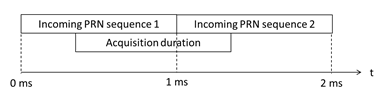
Figure 5.3: Acquisition - Integration duration.
As mentioned in PART 2, one navigation bit contains 20 PRN sequences and last 20 ms. As one does not know whether the acquisition process is aligned with an incoming PRN sequence, the acquisition might be carried out while there is a navigation bit transition. In that case, the result from the acquisition is erroneous and the receiver might consider that a satellite is not visible whereas it actually is (worst case when the navigation bit transition occurs at the middle of the acquisition process). To overcome this issue, the acquisition process is run twice on two successive milliseconds. By doing so, at least one acquisition iteration does not include any navigation transition bit.
Once the navigation bit transition has been taken care of, the acquisition is successful when a satellite is visible and one is provided with a coarse estimation of the carrier frequency of the GPS raw signal as well as its code phase. Nevertheless, the frequency error can be up to 250 Hz. Such an error cannot be handled by the PLL once the acquisition outputs are given as inputs to the tracking block. Consequently, the frequency estimation has to be refined. As the code phase is known with a good accuracy thanks to the acquisition, it is possible to remove it from the raw signal. If it is removed over 1 ms of the raw signal, there is no bit transition and only the carrier of the raw signal is left (see Figure 3.6 of PART 3). Then it is possible to refine the estimation of the carrier by computing the Fourier transform of the carrier.
The link and the figure below illustrate the front-panel of the Main_Acquisition VI.
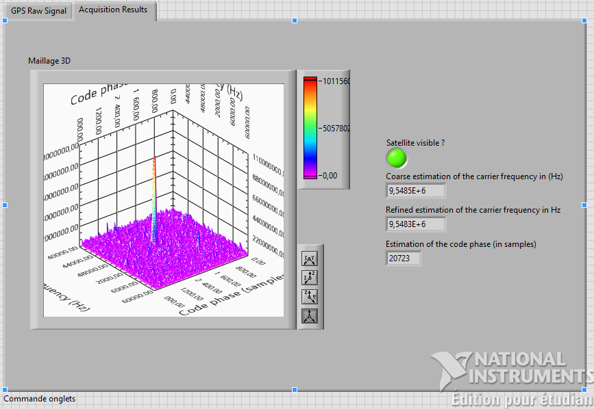
Figure 5.4: Acquisition results.
3 - Tracking.
See the UML Diagram of Section 2 under : Track.PNG
The files involved are :
- Main_Carrier_Tracking.vi : SnapTracking.png
- CalcLoopCoeff.vi : SnapCalcLoopCoeff.PNG
The theory of the PLL and DLL has been detailed in PART 3. In order to assess the carrier phase error and the code phase error, several discriminators can be used for the PLL and the DLL. The discriminators used for the PLL and the DLL are given in the following table:
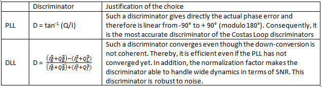
Table 5.1: Choice of PLL and DLL discriminators.
The DLL aims at updating the code phase of the locally generated PRN sequences for them to be perfectly aligned with the incoming PRN sequences. A PRN sequence is supposed to span over 1 ms. Therefore, the updating process of the DLL will be carried out over 1ms and the signal will be cut into slots of 1ms for the computation. Nonetheless, because of the Doppler shift that is induced by the motion of the satellite relatively to the receiver, the duration of an incoming PRN sequence might vary around 1 ms. Thus, a phase shift is introduced by that Doppler shift on the next millisecond to process. The DLL analyses this phase shift and adjusts the size of the window (=slot) for the next iteration. This way, the updating process vary around 1 ms and keep track of the code phase.
The following links and figure illustrate the front-panel of the Main_Tracking VI (/!\ The Main_Acquisition VI has to be run first in order to have the right inputs for the Main_Tracking VI).
Main_Tracking_1.PNG
Main_Tracking_2.PNG
Main_Tracking_3.PNG ![]()
Figure 5.5: Retrieved Signal at the output of the Tracking Block of the SDR GPS receiver.
4 - Navigation Data decoding.
- From this Section, the work that has been done is additional to the project.*
See the UML Diagram of Section 4 under : NavigationData.PNG.
a - Delimiting subframes.
The files involved are :
- FindPreamble.vi : SnapFindPreamble.png
- TestFindPreamble.vi : SnapTestFindPreamble.PNG
- GenerateFrame.vi : SnapGenerateFrame.png
- ParityCheck.vi : SnapParityCheck.png
findPreamble.vi finds the first preamble occurrence [1 -1 -1 -1 1 -1 1 1] in the bit stream of each channel. The preamble is verified by check of the spacing between preambles (6sec) and parity checking of the first two words in a subframe. At the same time function returns list of channels, that are in tracking state and with valid preambles in the nav data stream.
This program has been tested via TestFindPreamble.vi for an arbitrary frame and perfectly delimits the subframes as it is depicted :
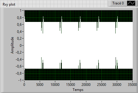
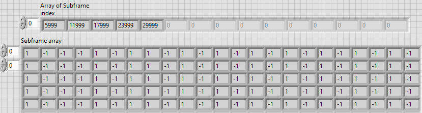
Figure 5.5 : Cross-correlation between arbitrary navigation frame and local preamble. Figure 5.6 : Subframes with index of delimitation.
Still for certain real signals, false alarm of preamble occurence is detected even with protection such as the parity check and the 6sec distance.
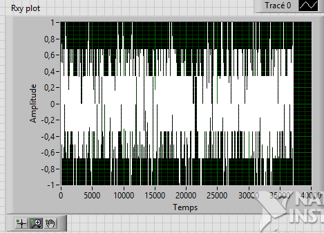
Figure 5.7 : Cross-correlation between real navigation frame and local preamble.
It prevents to find correctly the delimitation of the different subframes : refinement need to be implemented for such cases.
b- Decoding ephemeris and information within the frame.
The files involved are :
- Ephemeris.vi : SnapEphemeris.png
- BinaryArrayToDecimal.vi : SnapBinaryArrayToDecimal.PNG
- twosComp2dec.vi : SnapTwosComp2dec.PNG
- ParityCheck.vi_ : SnapParityCheck.png
- TestEphemeris.vi
Function Ephemeris.vi decodes ephemerides and TOW from the given bit stream. The stream (array) in the parameter Navigation bits must contain 1500 bits. The first element in the array must be the first bit of a subframe. The subframe ID of the first subframe in the array is not important.
Extracted ephemeris data are as mentionned in PART 4.
5 - Elementary blocks for localization.
See the UML Diagram of Section 5 under : Localization.PNG
a - Satellite position.
The files involved are :
- SatellitePosition.vi : SnapSatellitePosition.png
- TestSatellitePosition.vi : SnapTest_satellite_position.PNG
- Check_time.vi : SnapCheckTime.PNG
Computation of satellite coordinates X,Y,Z at TransmitTime for given ephemeris Ephemeris data. Coordinates are computed for one satellite by applying the algorithm of PART 4.
TestSatellitePosition.vi goal is to test SatellitePosition.vi with ephemeris data collected from GPS signal by University of Colorado [2] . The figure illustrates the computed satellite orbit level with respect to Earth radius level :
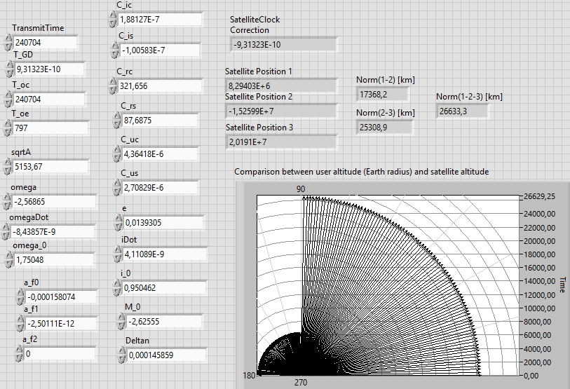
Figure 5.8 : Interface with ephemeris as input and illustration of the satellite position.
b - Pseudoranges.
The file involved is :
PseudorangesComputation.vi
PseudorangesComputation.vi finds relative pseudoranges for one satellite at the specified millisecond of the processed signal which has been stored in the file absoluteSample_sat(i).txt after the tracking function. The pseudoranges contain unknown receiver clock offset. It can be found by the least squares position search procedure in the following.
c - Least Square solution for position determination.
The files involved are :
- LeastSquarePosition.vi : SnapLeastSquare.png
- SatelliteRotationECEF.vi : SnapSatelliteRotationECEF.PNG
- toTopocentric.vi : SnaptoTopocentric.png
- CartesianToGeodetic.vi : SnapCartesianToGeodetic.png
- TroposphericCorrection.vi : SnapTropospheric.png
Function LeastSquarePosition.vi calculates the Least Square Solution based on the demonstration of PART 2 - Section 2.
Moreover it is also necessary to apply different change of coordinates system such as toTopocentric.vi , CartesianToGeodetic.vi and rotation SatelliteRotationECEF.vi
Finally, the tropospheric correction for pseudoranges accuracy is computed in this part.
Hint for coordinate systems :
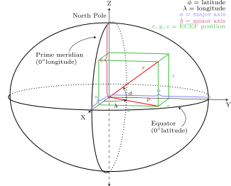
Figure 5.9 : ECEF (Earth-Centered, Earth-Fixed) coordinate system.

Figure 5.10 : Flattened Sphere for reference ellipsoid coordinates (Geodetic).
6 - Receiver position computation.
See the UML Diagram of Section 6 under : Receiver.PNG
The files involved are :
- ComputeReceiverPosition.vi : SnapReceiver.png
- NavigationProcess.vi : SnapNavigationProcess.png
- CartesianToGeodeticForUTM.vi : SnapCartesianToGeodeticForUTM.png
- CartesianToUTM.vi : SnapCartesianToUTM.png
For the sake of structuring, a block NavigationProcess.vi includes FindPreamble.vi , Ephemeris.vi , SatellitePosition.vi in order to fine-tuned the process for one satellite from frame delimitation to satellite position determination.
ComputeReceiverPosition.vi is the main VI . It combines navigation process of different satellite, loops on pseudoranges measurement points and deduces receiver position via Least Square VI and the associated DOP (Dilution Of Precisions).
Then, the receiver coordinates are converted into UTM coordinates with CartesianToGeodeticForUTM.vi and CartesianToUTM.vi
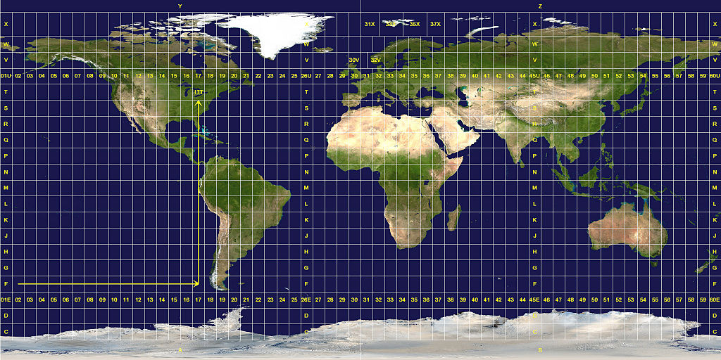
Hint for UTM coordinate system :
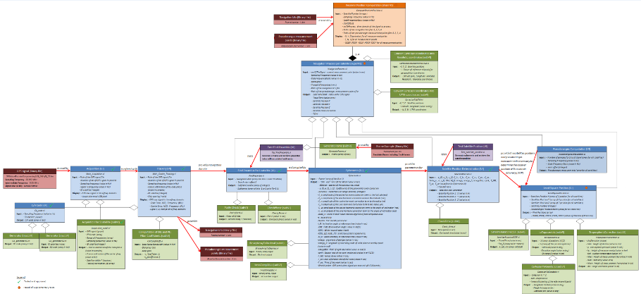
7 - Complete UML Diagram of the receiver.
The UML diagram with real size is available under : UMLDiagram.png
Here is a small overview of the structure :
References :
[1] K. Borre, D. M. Akos, N. Bertelsen, P. Rinder, S. H. Jensen, A software-defined GPS and GALILEO receiver
[2] http://www.colorado.edu/geography/gcraft/notes/gps/ephclock.html