
Receiving at the Lab
- Table of contents
- Receiving at the Lab
In order to test the whole radio communication chain, a receiver was set up on the laboratory, capable of receiving the RF signal emitted by the Cubesat, demodulating it, decoding the message and displaying it on real time.
The set-up
The reception of the signal at the laboratory is accomplished by using the architecture shown in the following scheme:
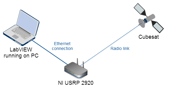
Figure 1: Receiver architecture
- A NI USRP 2920, an instrument capable of receiving radio signals, sampling them and sending the data to a computer (in this case, via Ethernet).
- A computer running LabVIEW, which handles the data acquisition via Ethernet, and is in charge of processing it afterwards (demodulation, decoding and display).
USRP
National Instruments manufactures a series of products called USRP (Universal Software Radio Peripheral), which consist on transceivers based on Software Defined Radio (SDR). The USRP is a widely used platform since it allows to perform RF prototyping in an easy and quick way, using only a PC running LabVIEW, without the need of extra equipment.
This equipment allows to perform both transmission and reception of RF signals. Regarding the transmission, it is possible to receive RF signals in a wide range of frequencies, and then sample them using a very fast SDR. The obtained data is stored in a buffer, until it is sent to a computer in frames of configurable size. The same is valid for transmission: the USRP is capable of receiving digital data, and then transmitting it via RF in a wide range of carrier frequencies.
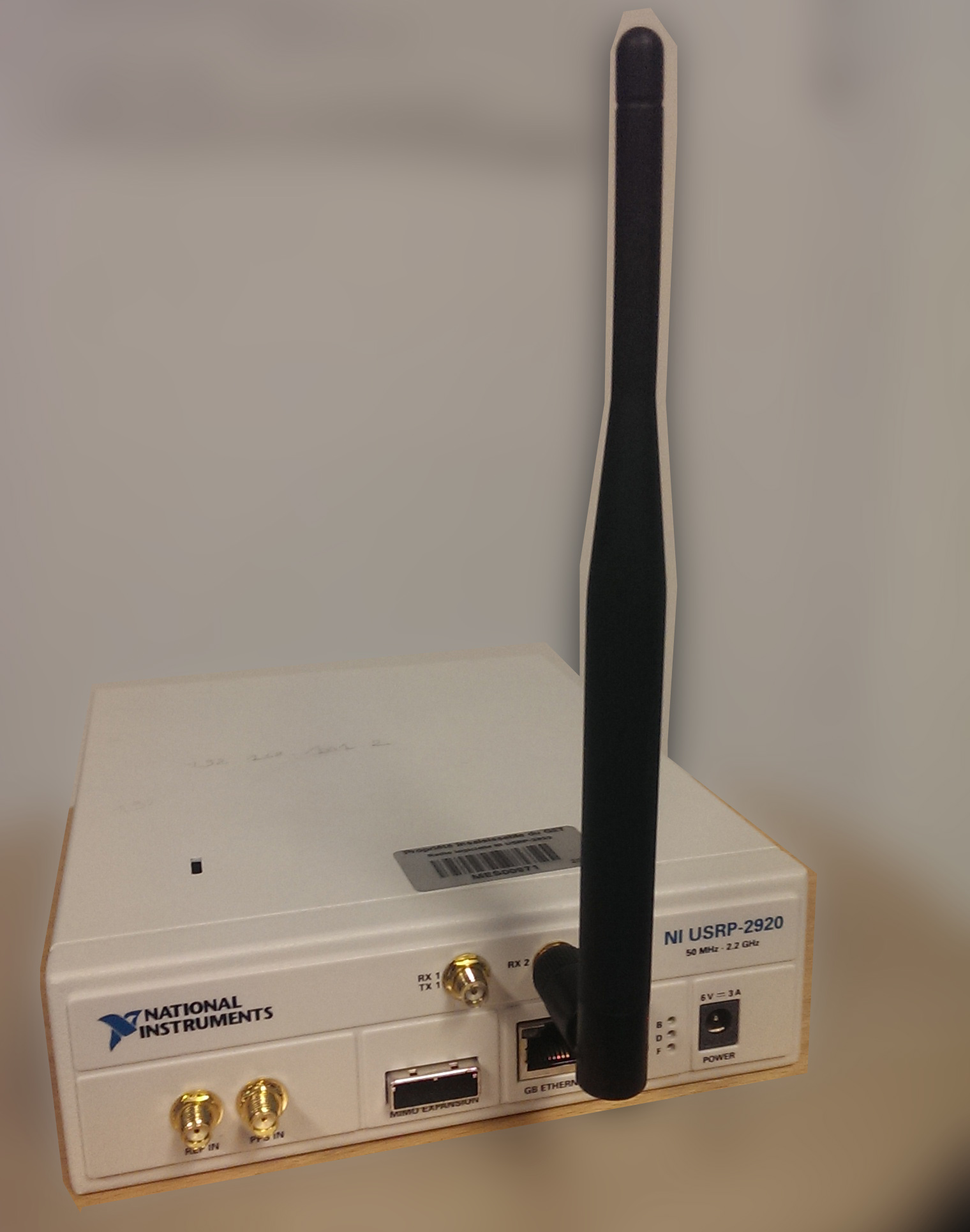
Figure 2: NI USRP-2920 at the lab
The model of the USRP used at the lab is the NI USRP-2920. This version works with a central frequency in the range from 50 MHz up to 2.2 GHz, covering the ISM, FM radio, GPS, GSM and radar bands. In particular, it covers the frequency used by the Cubesat, which is the 433 MHz ISM band.
The USRP-2920 is able to sample the signal and acquire I/Q (In-Phase and Quadrature) data with a rate ranging from 200ksamples/sec to 20 Msamples/sec, and send them via Ethernet with a speed of up to 25 Msamples/sec, to be processed with NI LabVIEW. The acquired I/Q samples can be used to demodulate different types of analog modulated signals (AM, FM or PM).
In the present case, the modulation used is BFSK (Binary Frequency Shift Keying), with a carrier frequency of 433 MHz, and frequency shift of +/- 20 KHz (a total shift of 40 KHz). In order to meet the Nyquist criterion and avoid aliasing, the sampling must be done at, at least, 80 KHz. The USRP amply meets this requirement.
The USRP acts as a host in a local network, and the communication with the computer is done over IP (the USRP has its own IP address). The interface is done directly with LabVIEW, which provides a set of modules required to work with this equipment (configuring and establishing a connection, data acquisition and transmission, etc). Once a connection is set up, the USRP sends the sampled data at request of LabVIEW.
The parameters needed to establish the connection, and successfully sample the radio signal are shown on the figure 3, where LabVIEW Front Panel is shown.
LabVIEW Virtual Instrument
![]() The software chosen to process the data is LabVIEW, of National Instruments, due to its compatibility with the USRP and to the simplicity with which the acquired data can be processed in order to obtain the message.
The software chosen to process the data is LabVIEW, of National Instruments, due to its compatibility with the USRP and to the simplicity with which the acquired data can be processed in order to obtain the message.
LabVIEW, a graphic programming platform, is ideal for measuring, processing and displaying data in real time. Unlike most common programming languages, which are for declarative programming (and basically state a sequence of instructions), LabVIEW is a data-driven programming language, and what describes is the processing to be done to the data. LabVIEW uses a graphical interface, in which the data is represented by lines, and the processing applied to it by different function blocks. Thus, by interconnecting the lines with the blocks the desired processing is achieved. All this makes LabVIEW more suitable for real time data processing than other alternatives. A LabVIEW program is divided into two parts: the Front Panel, and the Block Diagram.
The Front Panel
In LabVIEW, the interaction between the user and the program is done through the Front Panel. Here, the user can find all the parameters that can be set in order to control the execution, and also he can find all the important data displayed.
The developed front panel looks as follows:
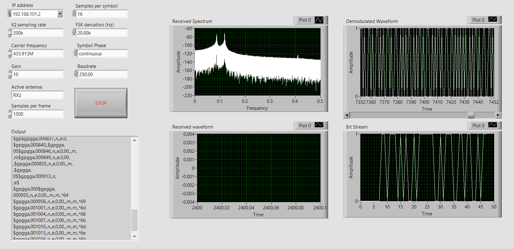
Figure 3: Front Panel of the LabVIEW Virtual Instrument
At the top, right-side, the user may find all the parameters that need to be set in order to correctly acquired and demodulate the data. The list of parameters to be set are:
- IP Address: IP address of the USRP.
- IQ Sampling Rate: Sampling rate of the signal. 200k is the minimum value.
- Carrier Frequency: Central frequency at which the USRP tunes. The frequency used here is the carrier frequency of the FSK.
- Gain: optional amplification of the signal. The default value is 0dB.
- Active antenna: the USRP counts with several antenna connectors. The one in use is RX2.
- Samples per frame: amount of samples per each Ethernet frame. This value should be small enough to give the impression of real time processing of the signal.
- Samples per symbol: the number of samples per FSK symbol to be used in the demodulation. The default value is 16.
- FSK deviation: the frequency shift between the Carrier Frequency and each of the two subcarriers. This value is equal to 20 KHz.
Below these parameters, a text box displays the messages obtained from the RF signal. The messages have the format described in Payload Integration page.

Figure 4: Close up of the Front Panel graphs.
- At top-left, the spectrum of the sampled signal is shown. This signal has been translated from the carrier frequency to the baseband and, is a complex signal, meaning that the spectrum will not be even. If well centered, both signal peaks (corresponding to the ON and OFF subcarriers) will superpose at 20 KHz.
- At bottom-left, the sampled IQ time signal is displayed. It can be seen the frequency shift when the symbol changes.
- At top-right, the signal shown is at the output of the FSK demodulator. Here, the input signal has been sampled and demodulated. The Manchester symbols and the sync signal can be seen.
- At bottom-right, the bit stream obtained from the above signal is displayed (after synchronizing, and translating the Manchester symbols into bits).
The Block Diagram
The LabVIEW Virtual Instrument is able to acquire and process the data in real time. This is achieved in the following manner: the program runs in a constant loop (until the stop button is pressed), which consists of two main parts: acquisition and processing. The acquisition is also done with an inner loop, each iteration receiving a frame of data from the USRP, and storing it in a vector variable. When a certain amount of data is stored , the loop is stopped. The vector length used, is 7 Msamples, corresponding to 35 seconds of signal at 200ksamples/s; enough time to capture a message sent by the emitter. Out of the loop, this data is processed. Before inputing it in the demodulator, the received signal is downsampled in order to work with a smaller amount of data, and make the further processing faster. This parameter can be set from the front panel, and the default value is 16 samples per symbol.
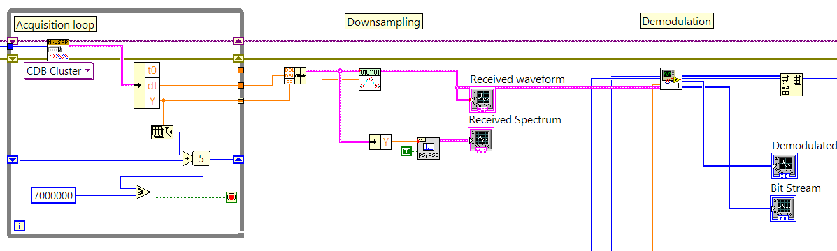
Figure 5: Main program loop, with acquisition loop, down sampling and demodulation.
The processing is done in a dedicated subVI, which takes as input the downsampled waveform, the number of samples per symbol and the frequency shift. A function block already made available by LabVIEW (available in the RF Modulation package) demodulates the signal, passing from an analog waveform to a stream of bits. This function takes also as input, matched filter and pulse-shaping filter coefficients, and they are used by the demodulator to sample at the optimum time. In the present case, both filters are rectangular windows (the same as the emitter side).
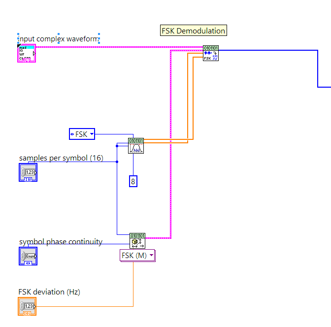
Figure 6: Signal demodulation.
The output signal is, however, not the information bit stream yet. This is due to the Manchester encoding performed to the bit stream at the transmitter side, where each bit was encoded as a rising or falling flank. In order to decode Manchester at the right point (there is an ambiguity regarding which flanks should be considered), a synchronization sequence is used: a burst of 14 ‘1’s. When a burst of more than 14 ones is detected, the Manchester decoding is synchronized.
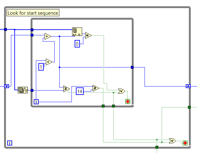
Figure 7: Loop in charge of looking for the sync sequence.
Once synchronized, the bits are taken in pairs. If a falling flank is detected, the information bit is a '1', and if a rising flank is detected, the bit is a '0'. If any of the other two forbidden combinations (two ones or two zeros) is detected, the translation is interrupted. This occurs when there is an error, or when the message has ended.
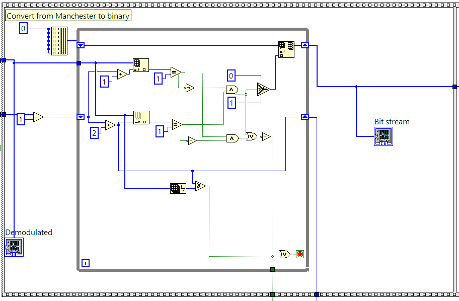
Figure 8: Part where the each Manchester symbol is translated into bits.
Finally, the next step is to remove the start and stop bits, and obtain each Baudot character. This is achieved by taking groups of seven bits, and removing the first (start) and last bit (stop). At last, each Baudot character is mapped to its associated ASCII character and displayed on screen, using two different look-up tables. Depending on which Baudot character mode is being transmitted, one table or the other is used. Each time a Shift to Letter, or Shift to Symbol is received, the mode is changed.
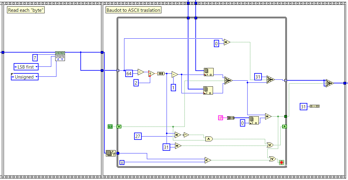
Figure 9: Part where the start and stop bits are removed, and the Baudot words translated into ASCII.
Results
The final results are shown in the text box, where the decode message is shown. Normally, when no errors are encountered, and the sync is successfully performed, the message obtained looks like the following:
$gpgga,124502,4333.8455,n,00128.5211,e,1,05,01.5,00131.5,m,049.8,m,,*47
In this case, there is position information available since enough satellites have been contacted, and the position obtained is 43º33´N, 1º28´E. When the GPS receiver obtains information from satellites, but not enough to do a trilateration, only the UTC time is shown. If no satellites are available at the moment, the GPS receiver may indicate the last obtained position if it is not too old.