Further improvements¶

As we have seen, the link budget equations can become very complex and, during the two months we have had to develop this project, sometimes we have had to do some assumptions in order to simplify the calculus and thus achieve a coherent software tool.

At the beginning of the project we did a long list of all possible options and features that could be included in a link budget tool, selecting them by order of priority in order to implement them.

Finally, in this last part is shown a list of other features and improvements that could be performed for future students.

SERVICE¶

- Increase the possibilities of $BER$ and corresponding $\frac{Eb}{No}$ and Code gains. Our possible modulation applied is based in a table of the situation of Quasi-error-Free. As seeing in the figure below, from [1].Quasi-error-free (QEF) means that we will have less than one uncorrected error event per hour, for this table this situations correspond to a PER (Packet error ratio - relative to the symbols) about $10^{-7}$ .

 
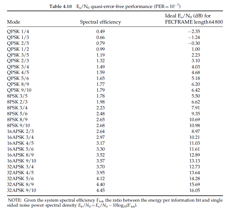
<div style="margin-left: auto; margin-right: auto; width: 30em">Figure 1 - Table applied in SatLinkTool, Quasi-error-free situation, from reference [1].
</div>

We would like to add others situations like the for a situation without FEC, when code rate = 1. We have already start this implementation. In the first steps we'we implemented, for QPSK,BPSK, 8PSK, 16PSK and 32PSK, the graphic of $BER$ x $\frac{Eb}{No}$. One idea, is take the value of $\frac{Eb}{No}$ from a user input of $BER$, and then, perform the calculations. This implementations in labview can be see below.

  <div style="margin-left: auto; margin-right: auto; width: 40em"> Figure 2 - Possible reference application to further increase of $BER$ possibilities </div>

To take the $\frac{Eb}{No}$ value from a $BER$ input, we can explore matlab functions like solve(x,y).

DOWNLINK¶

In downlink we have as an input, the $Tsky$ which can be assimilated as the the brightness temperature for the angle of elevation of the antenna, and for a frequency of downlink. As we done with th $ho$ value, which is take automatically by the input position of earth stations, in further improvements we can also help the user and automated the process to take $Tsky$ values using the following graphics. Probably this graphics can be obtained in ITU site or EUTELSAT in versions which we can manipulate with MATLAB. Then using the input values take it directly, in order to have one approximation nearer to the real implementation. In the figure 4, we can see the graphics which can be used to further improvement mentioned.

PAYLOAD¶

We have developed the first step to calculate the total depointing angle. It consist in the angles of satellite-earth station geometry angles $\alpha $, $\alpha$ *, $\beta$, $\beta$ * and true view angles($\theta$, $\varphi$)$. In the matlab code applied in this step we also have more useful information like the distance of the satellite to the Earth location $R$. values. One further improvement is finalize this implementation, performing the total depointing, and then the minimum antenna diameter of receiving Earth Station (ES B in Satlinktool). The pre-defined window for this implementation is the Depointing 2, located in Payload -> Antenna. This window is showed in figure 3, below:

 
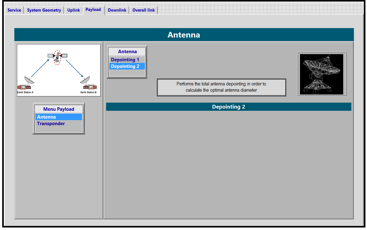
<div style="margin-left: auto; margin-right: auto; width: 30em"> Figure 3 - Pre-defined window to finalization of total depointing angle computing </div>
h1. REFERENCES

[1]