Tests and results
The aim of this part is to demonstrate the proper functioning of the tool. That is, the explanation of how we have shown that the results of all the link budget operations are correct, as well as that the tool is understandable for a user who has never used before.
For that purpose, different test with other students have been carried out. Thus, it has been possible to identify the difficulties of understanding of some aspects. For instance, we have identified some hesitation to understand well what refers each input parameter, and so we could take steps to correct it, and add more explanation in the popup help, or add some diagrams blocks in some tabs in order to have an extra visual aid of the correct placement of each parameter in the process.
Checking results
Below are shown the different verification carried out in each tab in order to verify the correct computation implementation.
Services
This tab was easy to verify because the few calculations that are performed there are a direct application of simple formulas, moreover in the book Satellite Communication Systems there are several tables with typical values to check the results. In addition, it was also verified with the values of Project 2.
System Geometry
In the Geometry tab are calculated basically three parameters: The distance between each earth station and the satellite (Range) and elevation and azimuth angles.
The Range is easily checked by placing both satellite and earth station in the latitudes and longitudes equal to 0, thus the range obtained will be equal to the altitude of the satellite orbit. As we are studying the case of a geostationary orbit this range corresponds to 35786 km.
To test the azimuth and elevation angles it has been used real cases with existing satellites and different places on Earth. For example, Eutelsat web (www.eutelsat.com) offers the possibility to make these calculations with the coordinates of one of its satellites. Thereby, figure 1 shows the elevation and azimuth angles obtained using the satellite "Eutelsat 10 A" (Geostationary satellite at latitude 10º East) with respect to two earth stations placed in Rome (Italy) and Palmeira (Brazil). Figure 2 shows that placing the same input values in the SatLinkTool we get the same results.
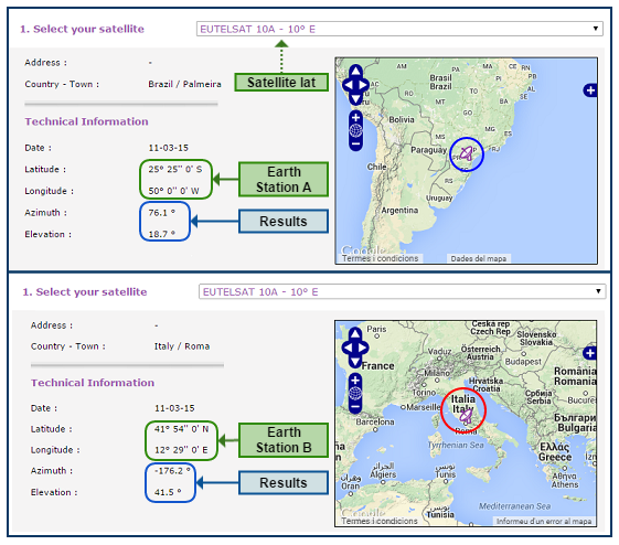
Figure 1: Parameters obtained on the Eutelsat web [1].
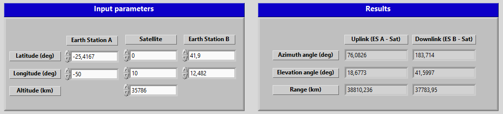
Figure 2: Parameters obtained using the SatLinkTool.
In Figure 3 it can be seen that the locations of the Earth stations obtained in the map shown on the System Geometry tab are also correct.
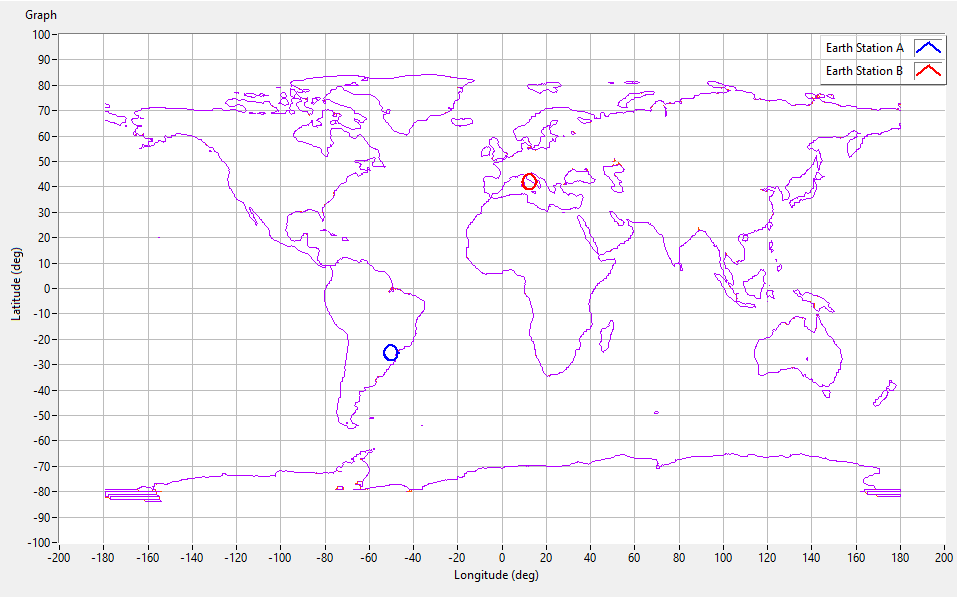
Figure 3: Position of the Earth Stations obtained in the System Geometry tab of the SatLinkTool.
Uplink
For checking the equations on the Uplink tab we have made several test using either some book values or the calculations of Project 2 or other exercises realized throughout the year in the courses of STEL.
Specifically, for the calculation in terms of clear sky conditions we have used the examples of the book ”Space Communication Systems” [2]: sections 5.4.2 (Example 1: Uplink received power) and 5.6.2 (Clear sky uplink performance), and checked that the results were exactly the same. For the case of rainy conditions we have tested both calculations of Project 2 and the values of section 5.7.4 (Link performance under rain conditions).
Payload
Antenna depointing 1
In the payload we have two windows menu. The first is the Antenna and the second the transponder. The window antenna, in turn, has the Depointing 1 and Depointing 2 window. Only the first calculations of depointing were performed in the application, being the total depointing angle computation, an additional feature to be performed in further implementations of the SatLinkTool. In these first calculations, we have performed the true view angles (θ, φ), the satellite antenna azimuth angle (α) and satellite antenna elevation angle (β), as well as two auxiliary angles α*, β*.
In order to check if our results were correct, we have compared, using the same inputs values, the results showed in an example of the "Satellite Communications Systems" book (page 496). The figure below shows the verification of these results.

<div style="margin-left: auto; margin-right: auto; width: 50em">Figure 4 - Comparison of results. In the left side the input values and results for SatlinkTool and in the right the input and results of an example of calculating, found in the book.
</div>
Transponder
In SatlinkTool we have transparent payload, with two forms of carriers per transponder: single carrier or multicarrier (only 3 carriers/ transponder was applied). The formulas used for each case are exposed below.
- Single Carrier
The input is the IBO value, which must be entered by the user, we can perform OBO and IM product equal to zero:
OBO|dB=IBO|dB+6−6⋅exp(IBO|dB6)
IM=0
(CN)IM|dB=inf
(CN)U,sat|dB=(CN)U|dB−IBO|dB
(CN)D,sat|dB=(CN)D|dB−OBO|dB
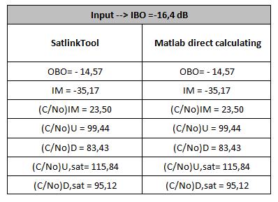
We have the following table of values, performed with the SatLinkTool compared with results of reference [1] examples, and compared with matlab script.

<div style="margin-left: auto; margin-right: auto; width: 25em">Table 1 - Comparison of results. For a IBO=-16.4 dB, matlab script ( download ) was used for to perform similar computing.
</div>
- Multi Carrier - Three carriers drive for transponder.
The input is the IBO value, which must be entered by the user, once we have IBO we can perform the following values:
=>OBO, => IM, => (CN)IM, => (CN)U,sat, => (CN)D,sat
OBO|dB=IBO|dB+6−6.4⋅exp(IBO|dB+66.4)
IM=3IBO|dB+17−6.25exp(IBO|dB+11.756.25)
(CN)IM|dB=OBO|dB−IM
(CN)U,sat|dB=(CN)U|dB−IBO|dB
(CN)D,sat|dB=(CN)D|dB−OBO|dB
We have the following table of values, performed with the SatLinkTool compared with matlab script.
<div style="margin-left: auto; margin-right: auto; width: 25em">Table2 - Comparison of results. For a IBO=-16.4 dB, matlab script (download ) was used for to perform similar computing.
</div>
Downlink
The checking process of the equations on the Downlink tab are similar as the ones done in the Uplink tab. In this case, for the calculation in terms of clear sky conditions we also have used some examples of the book ”Space Communication Systems” [2] : sections 5.4.3 (Example 2: Downlink received power) and 5.6.3 (Clear sky downlink performance), and we also checked that the results were the same. For the case of rainy conditions we also have test both calculations of Project 2 and the values of section 5.7.4 (Link performance under rain conditions).
Overall link
Finally in the overall tab basically a compilation of the main parameters obtained in the previous tabs is done and then it is easy to calculate the (C/N)T and available margin, the results were checked with exercises done in class during the course as well as the results obtained in Project 2.
References
[1] www.eutelsat.com/deploy_SorbamLight/pages/azimuthElevation.do?action=calculate
[2] Maral, Gérald / Bousquet, Michel. Satellite Communication System.-5th ed. UK, 2009.
