Implementation¶

• Table of contents
• Implementation
  • Diagram block of application development
  • Overview Application Plan
  • Preliminary design
  • Added features
    • Control Features
  • Final design
    • Service:
    • System Geometry:
    • Uplink:
    • Payload:
    • Downlink:
    • Overall link:
  • Validation & Final tests
  • Delivery Application
• REFERENCES

At this point we were familiar with the system analyse of a link budget, knowledge acquired throughout the different subjects imparted in the master course and especially thanks to the realisation of the project 2 (Design of a regional multi-beam satellite system), that has an strong bond with the present project.

Diagram block of application development¶

The diagram below shows the planning with the different phases we have designed in order to perform the successful and coherent development of the tool.

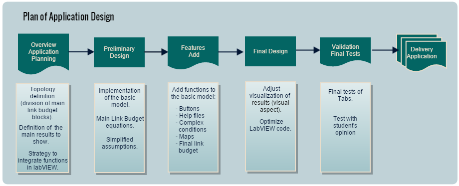
<div style="margin-left: auto; margin-right: auto; width: 25em">Figure 1: Project plan diagram.
</div>

In short, the first steps were to decide what would be the basic structure of our link budget program and identify all the parameters and possible calculations, as well as the logical place to perform them in this structure. Thus, a preliminary design with the fundamental and simplest conditions has been performed, to then add gradually other features in order to improve its capabilities. Finally, verification of results and testing with subjects has been done in order to finish the complete design of the tool. These steps are further explained below.

Overview Application Plan¶

At the beginning of this project it was essential to ask ourselves about what we would expect of tool a Link Budget Tool. For instance, some thoughts we considered were: If I had an analysis tool... what would I do with it? What would be the settings I give? What would be the results that I expect?

Hence, in order to design a tool to help with the comprehension of the link budget analysis, we have had to ask each time the question "How will I present my results and information?”. This leads us to the GUI (Graphical User Interface), one of the key points of this project.

When we thought about all this aspects, we know what it has to do, which are the necessary parameters and results we want to show, etc. At this point, we can start to design our screen according to this. Thus, we identified the topology of the satellite communication system and we divided it in the following block groups, that corresponds to different tabs in the software tool:

• Service: The user introduces the requirements of his system (i.e. modulation, channel BW, code rate, margin, etc.), and the tool gives as outputs the required information bit rate, overall link carrier-to-power noise power ratio, etc.

• System Geometry: The user introduces the latitude and longitude of the earth stations and the satellite and he obtains as outputs the corresponding azimuth and elevation angles and the range between satellite and each earth station.

• Uplink: The user introduces all the parameters involved from the transmission on earth station A to the reception at the satellite, including the uplink path losses depending on the weather conditions. All the results associated with uplink are computed, being the uplink carrier-to-power noise spectral density the most important result.

• Payload: The user introduces the input back-off and the carrier-to-power intermodulation power ratio is computed.

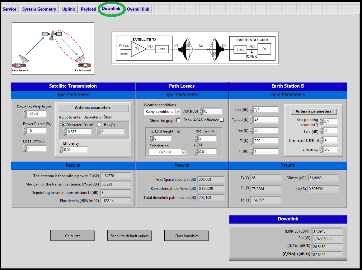
• Downlink: Similar to uplink, but here the parameters introduced by the user are those involved from the satellite transmission to the reception on earth station B.

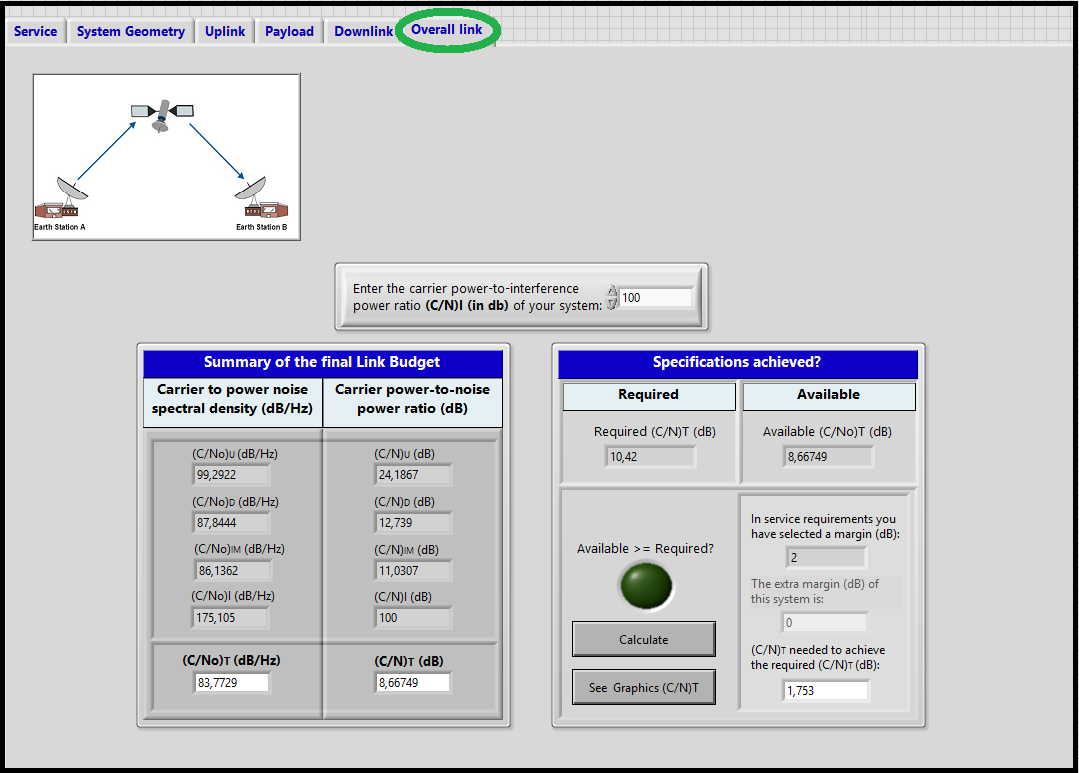
• Overall link: The user can see a summary of the principle results obtained in the previous tabs and introducing the carrier power-to-interference power ratio of the system the tool determines if the link budget requirements are achieved with the given specifications or not.

Preliminary design¶

It is known that link budget equations can become messy and complex and this calculus involve several aspects and conditions, furthermore, link budget can be analysed from different points of view. Globally, it can be defined with the following approaches:

• The first approach is a feasibility study: The user gives the features of the system, the targeted service, the bit rate, the bit error rate, etc., and the link budget says either if it is possible with this margin or if this is not possible (negative margin).

• In the second approach the user also defines the features of the system, and then the link budget says what is possible to do in terms of bit rate, bit error rate, etc.

• Finally there is a third approach where the user says which is the service he would like to have, and the link budget tool finds all the system settings. But this approach is much more complex, because as there are several parameters to define, it turns into a lot of different configuration options.

In the interest of simplification we have implemented the link budget using the first approach: the feasibility study.

Thus, once defined what would be the program structure, we started implementing the calculations starting from a first basic implementation. I.e. calculating the basic parameters for each tab and taking the simplest hypothesis (e.g. clear sky conditions rather than rain conditions), and finally by assembling the individual results for the overall link budget.

At this early stage we had a first implementation, comprehensive and simplified, but only with the numerical values. From here we started, in the one hand, to focus on the visual and clear interface aspect of the program and, in the second hand, to add more complex equations and conditions, as well as new LabVIEW features that are listed below.

Added features¶

• Service
  • Multicarrier/Singlecarrier
    This feature allows to select between a multicarrier and singlecarrier mode. If the singlecarrier is selected, there will be one carrier per transponder, which means that all transponder Bandwith will be used only by this carrier. In multicarrier mode, we have implemented the option of 3 carrier per transponder. Then the transponder BW will be divided by 3, and we'll have different formulas to compute the IBO, OBO. In multicarrier there will be an inter modulation product and ${(C/No)}_{IM}$ that will affect the available ${(C/No)}_{T}$. When a mode is selected the payload transponder window will use the corresponding formulas, the mode will also be indicated in the payload transponder window, in a dialog box.
  • Selection of BER (Quasi-error-free , $BER=10^{-7}$).
    The SatLinkTool was firstly designed to take in account modulations, with a range of code rates, in the situation of Quasi-error-free. Each code rate imposes a code gain in comparison with the "no coding" situation. In service, the user can select a modulation (BPSK,QPSK,8PSK, 16PSK,32PSK), the channel Bandwith, and the mode (single/Multicarrier), and, in accordance with this inputs, a required ${(C/N)}_{T}$ is generated. This latter value, will be compared, after all path calculations, will the available ${(C/N)}_{T}$. A table with all possible code rates and modulations for the application is showed in Further Improvements.

 
<div style="margin-left: auto; margin-right: auto; width: 25em">Figure 2- service features.
</div>

• System Geometry
  In system geometry we have added a map with indicates the position of the two stations (A and B ). This map has the objective to situate the user with in according of the input latitude and longitude.

• Payload
  • Depointing 1
    One of more exhaustive calculated is related to the optimal antenna diameter. To perform this value, we have to calculate the total depointing angle. In the Depointing 1 window the angles of the geometry satellite-Earth Station B( Downlink station) are computing. The aim of this computation is provide a first step to the total depointing angle calculate. This calculation take the values of the Satellite and Earth Station B position from the window System Geometry. Then, if the user want change the input parameters, it is necessary to go to the System Geometry window, set them, and recalculate.
  • Transponder
    The payload chosen to be used in this application is the Transparent payload. As mentioned before, two modes are provides multi/single carrier. The transponder window perform, from an $IBO$ input, $OBO$, intermodulation product,${(C/No)}_{IM}$ , and $(C/No)sat$ values related.
• Uplink/ Downlink
  • Clear Sky or Rain condition
    The main features implemented in uplink downlink is the possibility to choose between clear sky and rain conditions. The user can also specify the losses of the system (Path loss: gas attenuation, rainfall rate, exceed percentual) in according with the Earth Station position, and Earth station Loss (Noise temperature of feeder, Tground etc). The main values of link budget ${(C/No)}_{U,D}$, $EIRP$, $G/T$ are the outputs of each individual path (uplink: Earth Station A => Satellite, downlink: Satellite => Earth Station B).
    In rain conditions there is the possibility to see a map with the $R001$ values in according with Earth Station position.This graphic is interesting to have an idea of what can be the coherent values of $R001$ to choose.
  • $h0$ - Yearly average 0°C isotherm height(km) above sea level (value used to compute the effect of rain conditions), is done automatically by the locations of the Earth Stations. For each one, the link budget uses an ITU Recommendation
    table, with, for a input of longitude and latitude, gives the correspondent $ho$ - value. The table of values is based on the graphic below:

 
<div style="margin-left: auto; margin-right: auto; width: 50em">Figure 3 - $ho$ table Yearly average 0°C isotherm height(km) above sea level . From ITU-R P.839-4 ("Download zip source"http://www.itu.int/dms_pubrec/itu-r/rec/p/R-REC-P.839-4-201309-I!!ZIP-E.zip)
</div>

• Overal Link
  • Required Objective accomplished - Indicator
    We have implemented one "led" indicator which signalize if with the modulation, carrier mode, and code rate specified in the Service window, our system is capable/or not to accomplished the ${C/N}_T$ Required.
  • Graphic of ${C/N}_T$ comparison
    This graphic have the comparison of the values obtained by our system ${C/N}_T$ Available in comparison with the ${C/N}_T$ Required . It's a final result for the user. This results can be appear like the three situations as show in the picture below.
    • In the first situation the system achieved the required ${C/N}_T$ for the modulation input in the Service window. In blue we have the available ${C/N}_T$, in red the required ${C/N}_T$ and in green the extra margin of our system.
    • In the second situation the system not achieved the required ${C/N}_T$ for the modulation input in the Service window, in yellow we have the needed ${C/N}_T$ to achieve the required. In this situation the available ${C/N}_T$ is greater than zero.
    • In the third situation the system also not achieved the required ${C/N}_T$ for the modulation specified, in yellow we have the needed ${C/N}_T$ to achieve the required. Notice that in this situation the available ${C/N}_T$ is lower than zero, which means that the linear value of the available ${C/N}_T$ is lower than 1. (corresponding to a situation with great attenuation due to loss).

 
<div style="margin-left: auto; margin-right: auto; width: 70em">Figure 4- Comparison of ${(C/N)}_T$ Required and ${(C/N)}_T$ Avaiable with the "led" indicator of accomplishment of system requirements with the modulation chosen.
Three situations:

• First ${(C/N)}_T$ avaiable$>$ ${(C/N)}_T$
• Second situation ${(C/N)}_T$ avaiable$<$ ${(C/N)}_T$ required, and ${(C/N)}_T$ avaiable > 0dB
• Third situation ${(C/N)}_T$ avaiable$<$ ${(C/N)}_T$ required, and ${(C/N)}_T$ avaiable < 0 dB.</div>

Control Features¶

We have add the following control features:
(v) Button "CLEAR VARIABLES" 
Clear all input variables of the window.
(v) Button "SET TO DEFAULT" 
Set all input variables of the window to default values (established taking in account examples of ref[1]).
(v) Button "CALCULATE" 
Compute the calculation taking the input values and providing the output (results).
(?) Information Pictures
In order to well understand and has an idea to the possibles values of the input parameters
(?) Help text
Each button, input parameter or result has an explanation in help labVIEW window.

Final design¶

In Figures 2 to 8 are shown the captures with the final design of each of the different tabs of the SatToolLink.

Service:¶

 
<div style="margin-left: auto; margin-right: auto; width: 30em">Figure 2: First window of SatlinkTool - Service.
</div>

System Geometry:¶

 
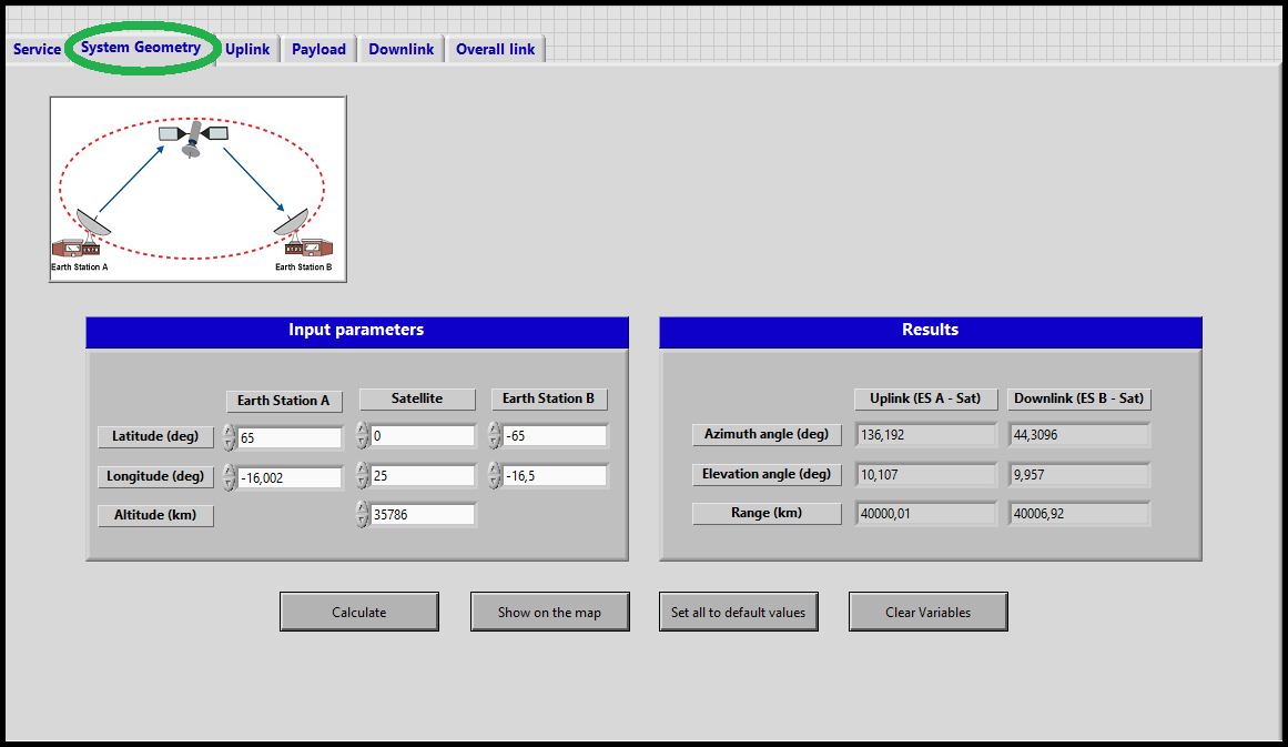
<div style="margin-left: auto; margin-right: auto; width: 30em">Figure 3: Second window of SatlinkTool - System Geometry.
</div>

Uplink:¶

 
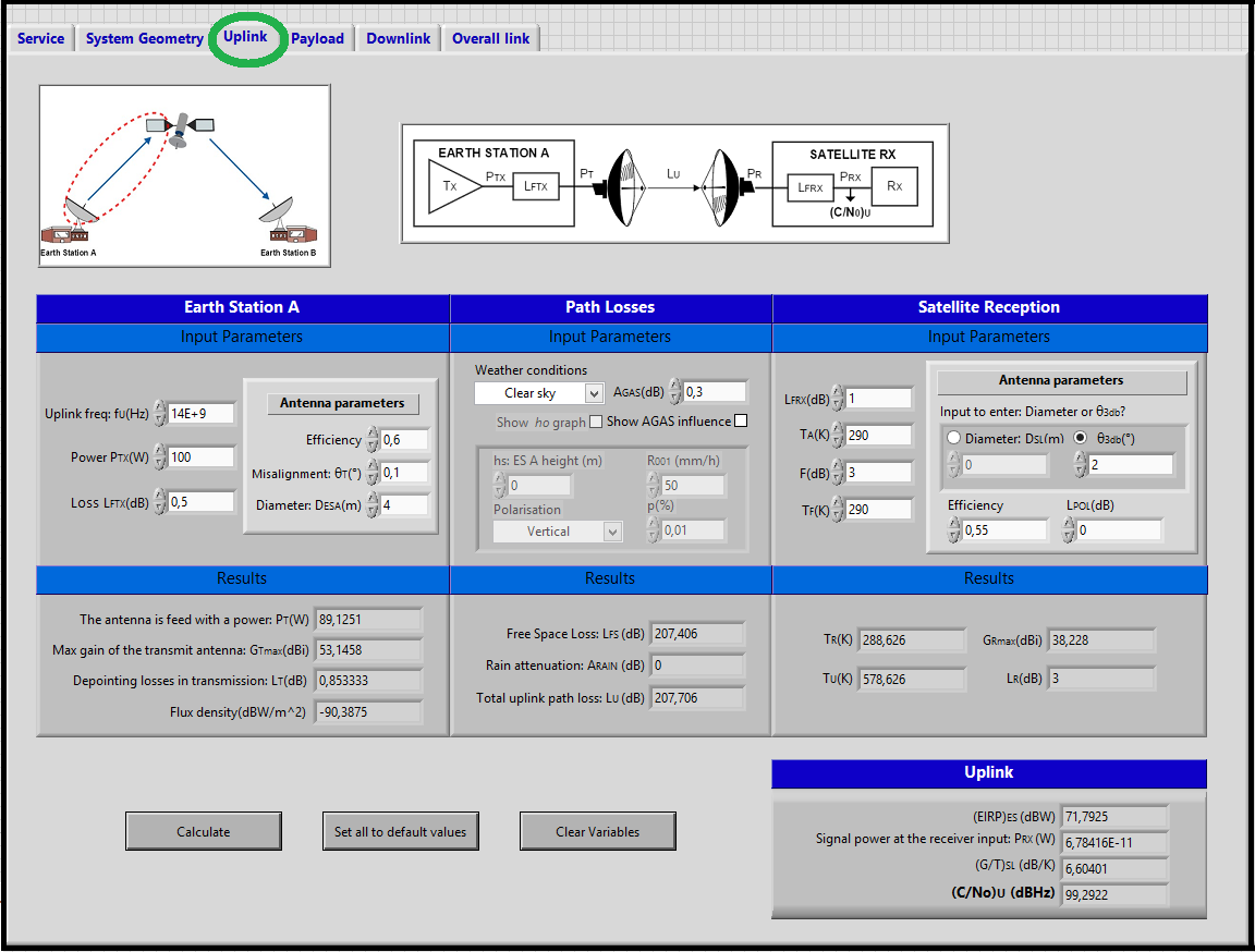
<div style="margin-left: auto; margin-right: auto; width: 25em">Figure 4: Third window of SatlinkTool - Uplink.
</div>

Payload:¶

• Transponder window:

 
<div style="margin-left: auto; margin-right: auto; width: 30em">Figure 5: Fourth window of SatlinkTool - Payload: Transponder.
</div>

• Antenna window:

 
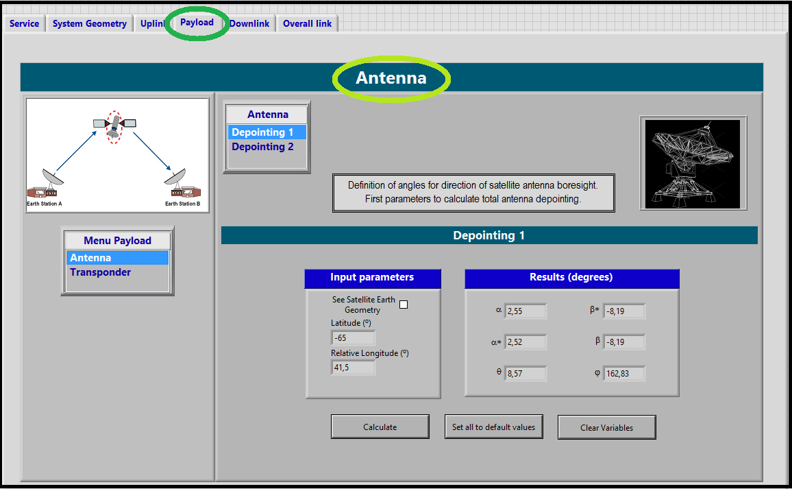
<div style="margin-left: auto; margin-right: auto; width: 30em">Figure 6: Fourth window of SatlinkTool - Payload: Antenna.
</div>

Downlink:¶

 
<div style="margin-left: auto; margin-right: auto; width: 25em">Figure 7: Fifth window of SatlinkTool - Downlink.
</div>

Overall link:¶

 
<div style="margin-left: auto; margin-right: auto; width: 25em">Figure 8: Sixth window of SatlinkTool - Downlink.
</div>

Finally, the figure below (Figure 8) shows the window where the user will have to attach the files needed for the correct functioning of the SatLinkTool.

• map.txt: File needed to show the map with the two earth station locations corresponding to the parameters entered in the System Geometry tab.
• h01.txt and h02.txt: These files are used when the Rain Condition is selected either in the Uplink tab or the Downlink tab in order to compute the 0 degree isotherm height (see section Added Features above for more information) [1].

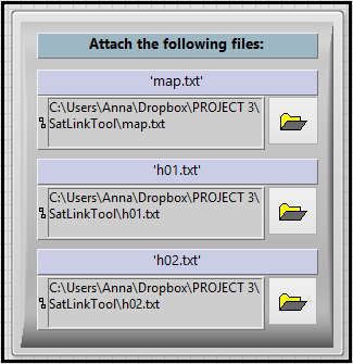
<div style="margin-left: auto; margin-right: auto; width: 20em">Figure 9: Attach file window of SatlinkTool.
</div>

Validation & Final tests¶

As the calculations were implemented in the different tabs, the results were also checked. Finally, once all the SatLinkTool design and implementation was completed, all tests were remade in order to verify the correct results. Tests with other students were also made in order to verify if the operation program was understood. This allowed us to detect the weak points of the tool and where we should modify the design or add additional explanation in the help pop-up. These steps are more detailed in section Tests and results.

Delivery Application¶

SatLinkTool is intended to be distributed out of charge through the website of the SCS program for future students. The files needed to use this tool are the following:

• File name: SatLinkTool.vi - File format: LabVIEW Instrument (.vi)
• File name: map.txt - File format: Text file (.txt)
• File name: h01.txt - File format: Text file (.txt)
• File name: h02.txt - File format: Text file (.txt)

A user manual of the SatLinkTool Software is also provided in order to support the users for the correct understanding of the tool and the process to follow. The User Manual is presented here.

REFERENCES¶

[1] Rec. ITU-R P.839-4 {UPDATE} Para el cálculo de h0